Fig. 02 — Signal dossier / 2026.10
Quantum Leap: AI-Driven Circuit Optimization
AI-driven quantum circuit optimization uses machine learning to cut gate counts and circuit depth, making today's noisy quantum hardware far more practical.
- Published
- 21 Oct 2026signal no. 02
- Category
- Quantum Computingfield note
- Read time
- 26 min~5686 words
- Topics
- Quantum Computing+ 3 more
- Author
- Trisham Patilindependent reading
Filed 2026-10-21 Signal no. 02Quantum Computing Read time: 26 min
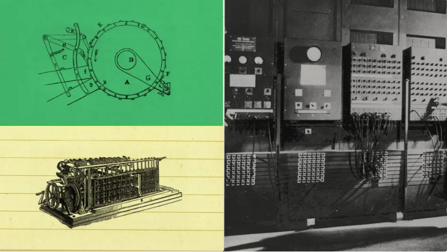
Quantum at the Edge: The Hardware Constraints Standing Between Us and Scalable Computing
Quantum hardware is stuck in a brutal engineering tug-of-war. It has to protect fragile quantum states from the environment while also scaling past a few thousand physical qubits.
The mainstream players (IBM, Google, Quantinuum) rely on noisy intermediate-scale quantum (NISQ) architectures with heavy error correction. Microsoft has made a fundamentally different bet: topological qubits built from Majorana zero modes.
The roadblocks look different depending on which path you look at, Microsoft’s topological one or the one the rest of the industry is on.
1. The Majorana / Topological Bottleneck (Microsoft)
Microsoft is trying to build a hardware-level immune system against errors. The idea is to split electrons in half into non-Abelian anyons. Information is then stored non-locally, so local environmental noise shouldn’t be able to disrupt it.
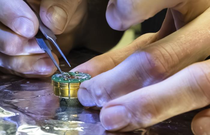
Researchers connect wires to a topological insulator–superconductor interface, the kind of hybrid material stack Majorana qubits depend on. Photo: Oak Ridge National Laboratory, CC BY 2.0, via Wikimedia Commons.

The physics and materials science wall. Clean Majorana zero modes need exact hybrid semiconductor–superconductor material stacks. The field is shifting from older aluminum setups to newer lead-based systems to widen the “topological gap”.
Growing crystals with zero structural defects at the atomic scale is violently difficult.
The “is it real?” skepticism. For years, the core constraint wasn’t just engineering. It was verification.
Physicists have heavily debated whether the signals measured in nanowires really are topological Majorana modes. They could also be conventional condensed-matter artifacts, such as trivial Andreev bound states.
Microsoft has reported major stability milestones, such as extended parity lifetimes in Majorana 2. Even so, clean, controllable braiding of these modes to execute actual quantum gates is still a monumental hurdle.
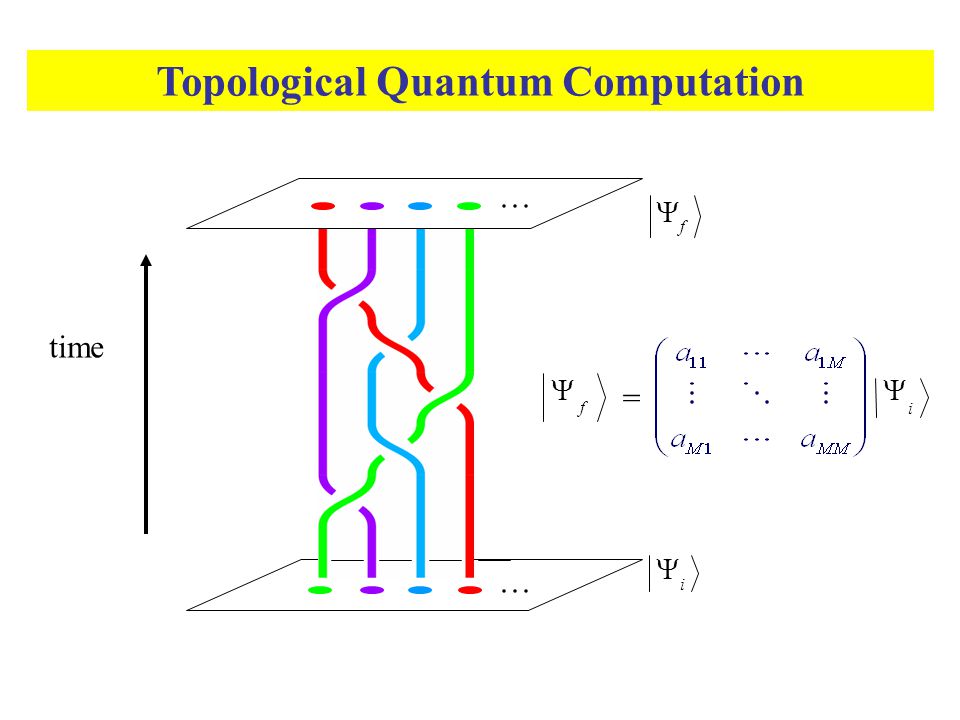
Braiding: anyons are swapped around each other over time, and the braid pattern itself is the quantum gate. Because the result depends only on the topology of the braid, small local wobbles shouldn’t change it. Diagram: CC BY 3.0, via Wikimedia Commons.

2. Universal Quantum Hardware Bottlenecks (Superconducting, Neutral Atoms, Trapped Ions)
For the rest of the hardware ecosystem, the constraints come from classical physics getting in the way of quantum mechanics.
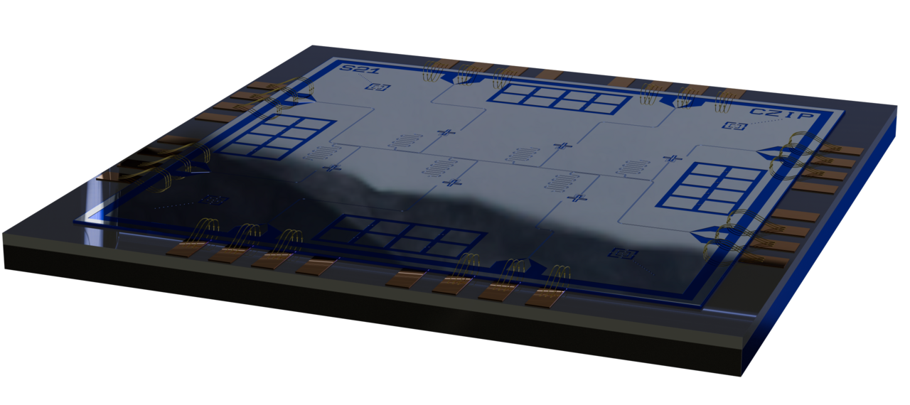
A superconducting quantum chip with six transmon qubits, wire-bonded to its control lines. Render: OJB Quantum, CC BY 4.0, via Wikimedia Commons.

The Decoherence and Error Wall
Qubits are hyper-sensitive. Stray magnetic fields, thermal noise and cosmic rays cause decoherence: qubits lose their superposition within microseconds to milliseconds.
Typical gate error rates sit around $0.1\%$ to $1\%$. Deep algorithms like Shor’s need logical error rates down to roughly $10^{-6}$.
Closing that gap takes thousands of physical qubits just to back up one error-corrected logical qubit.
The Cryogenic Wiring and Crosstalk Nightmare
Qubits have to run at millikelvin temperatures ($\sim 0.015\text{ K}$) inside dilution refrigerators. Without that, thermal energy destroys the quantum states.
But every single qubit needs its own control lines and coaxial cables. As you scale from hundreds to thousands of qubits, that wiring brings massive heat loads into the fridge.
It also causes crosstalk: unwanted electromagnetic coupling, where operating one qubit accidentally perturbs its neighbors.
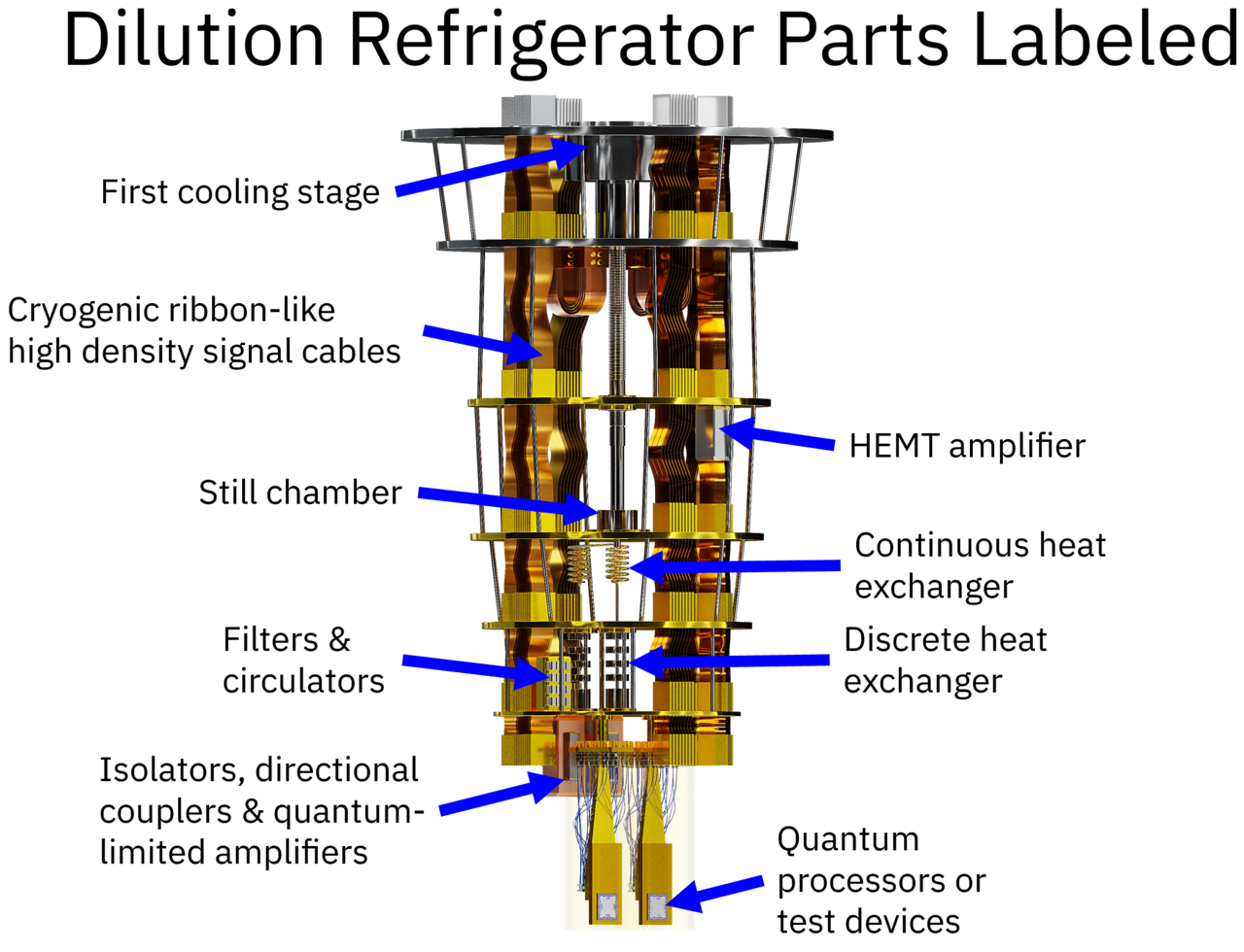
Inside a dilution refrigerator. Every stage down to the processor has to carry signal cabling, and every cable leaks heat into the coldest stages. Render: OJB Quantum, CC BY 4.0, via Wikimedia Commons.

Connectivity and Routing Limits
On standard 2D-grid superconducting chips, qubits can only talk to their immediate neighbors. If qubit 1 needs to interact with qubit 50, its state has to be routed through a cascade of SWAP gates.
Every extra gate injects more error into the circuit, and the calculation can lose its fidelity before it finishes.
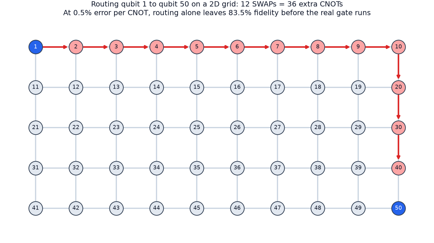
On a 5 × 10 grid, bringing qubit 1 next to qubit 50 takes 12 SWAPs. Each SWAP compiles to 3 CNOTs. At 0.5% error per CNOT, the routing alone costs about 16% of the circuit’s fidelity before the gate you actually wanted has run.
The Bottom Line
The industry has largely moved past just stacking up raw physical qubit counts.
The bottleneck is no longer abstract math. It is a brutal intersection of nanoscale materials engineering, cryogenic thermodynamic limits and fault-tolerant error-correction overhead.
Can AI Engineer the Future of Quantum Computing?
Quantum computers will need carefully designed circuits to run useful algorithms on limited hardware. That makes circuit design a natural test for AI-driven quantum circuit optimization.
Anthropic researchers gave Claude plain-language specifications for eight such circuits. The tasks came from chemistry, optimization, physics simulation and number theory. Claude also got an automated evaluator that checks and scores each design.
Working largely on its own, Claude found designs that improve on the best published circuits, in some cases by an order of magnitude or more.
Improvements like these substantially reduce the quantum resources that useful applications require. So practical quantum computers could arrive sooner than previously anticipated.
The work was led by Andi Gu as part of Anthropic’s STEM Fellows Program, with mentorship from Alek Kemeny, a quantum physicist at Anthropic. It was done in collaboration with Susanne Yelin (Harvard University) and Mikhail Lukin (Harvard University and QuEra Computing).
Read the full paper on arXiv: Discovering state-of-the-art quantum circuits with large language models (Gu, Kemeny, Yelin and Lukin, 2026).
The Quantum Bottleneck: Can Claude Shrink the Cost of Quantum Computing?
The hardware section described the walls. This section covers the other side of the problem: the cost of running an algorithm. Shrinking that cost turns out to be a circuit-design problem, which is exactly what AI-driven quantum circuit optimization can attack.
To see why, we need three pieces: what a qubit is, what an algorithm “costs” on a quantum computer, and one benchmark molecule the whole field uses to track progress.
Bits vs Qubits: What Makes Quantum Computers Different
A classical computer stores information in bits. Each bit is exactly 0 or exactly 1.
A quantum computer stores information in qubits. A qubit can be built from a single atom, a tiny superconducting circuit or a particle of light (a photon).
What makes a qubit different is superposition. Instead of being 0 or 1, it can sit in a weighted combination of both, written $\alpha\vert 0\rangle + \beta\vert 1\rangle$. Measure it and you get 0 with probability $\vert\alpha\vert^2$, or 1 with probability $\vert\beta\vert^2$.
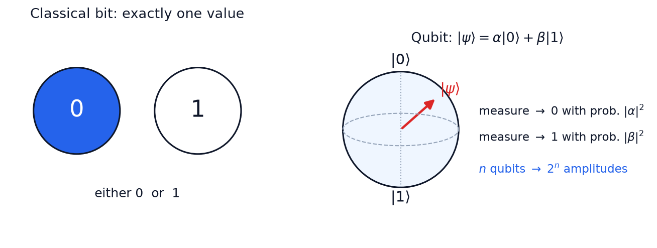
A bit is a switch. A qubit is a point on a sphere, and measuring it turns its amplitudes into probabilities. With $n$ qubits, the machine tracks $2^n$ amplitudes at once.
That exponential state space is the whole point. Some problems in chemistry, materials science and number theory are out of reach for classical machines precisely because the number of possibilities explodes. A quantum computer can, in principle, work with those possibilities natively.
Why Today’s Quantum Computers Can’t Run the Useful Algorithms Yet
Two things stand in the way, and both come straight from the hardware section.
Too few qubits. The machines built so far have hundreds to a few thousand qubits. Many of the algorithms with a real, practical advantage over classical computers need far more, especially once error correction is added.
Too much noise. Heat, vibration and even cosmic rays nudge qubit states. Each nudge is small, but they accumulate over a long computation until the final answer is wrong.
So qubits are scarce, and so is computing time, because the longer a computation runs, the more errors pile up. That turns algorithm design into a budgeting problem: use fewer qubits and finish in fewer steps.
How Quantum Algorithms Are Costed: Gates and the Toffoli Count
A quantum program, like a classical one, is a long sequence of simple operations. On a quantum computer these operations are called gates, and a diagram of gates acting on qubits is a quantum circuit.
Gates are not equally expensive. On a fault-tolerant (error-corrected) machine, most common gates are cheap. The costly ones are the “non-Clifford” gates such as the T gate. Each one has to be fed by a specially prepared “magic state”, produced in dedicated distillation factories that eat up both qubits and time.
The Toffoli gate is the workhorse expensive gate. It is a controlled-controlled-NOT: it flips a target qubit only when both control qubits are 1. That makes it the quantum, reversible version of a logical AND.
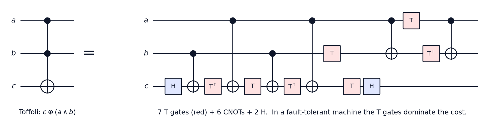
One Toffoli gate (left), built from cheaper gates (right). The textbook version needs 7 T gates. Tricks with extra helper qubits bring that down to 4, but it stays the expensive part. I checked numerically that this circuit equals a Toffoli exactly.
Because Toffoli gates dominate the runtime, the field uses the Toffoli count as its standard estimate of how long a computation will take. Together with the qubit count, it is the number every circuit optimization tries to shrink.
FeMoco: The Benchmark Molecule for Quantum Chemistry
The clearest illustration of this cost problem is a molecule called FeMoco.
FeMoco is the iron–sulfur cluster at the heart of nitrogenase, the enzyme bacteria use to turn nitrogen from the air into ammonia at room temperature. Industry does the same job with the Haber–Bosch process, which needs high heat and pressure and is commonly estimated to use 1–2% of the world’s energy.
If chemists understood exactly how FeMoco works, they could design better industrial catalysts, the substances that speed up chemical reactions. Classical computers can’t simulate it accurately, because its electrons are too strongly correlated. That is exactly the kind of problem quantum computers are meant to solve.
How a Quantum Computer Computes a Ground-State Energy
The key quantity is FeMoco’s ground-state energy: the energy of its most stable configuration. Chemists need it to predict how the molecule reacts.
The standard quantum algorithm for this is quantum phase estimation (QPE).
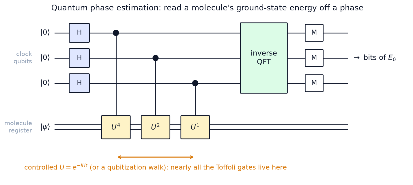
QPE in three moves: put the clock qubits in superposition, run controlled evolutions of the molecule, then use an inverse quantum Fourier transform to read the energy out as binary digits.
The steps are:
- Prepare the molecule register in a state close to the ground state.
- Evolve it under its own Hamiltonian, controlled by a set of “clock” qubits. Each clock qubit triggers twice as much evolution as the one below it, so the energy gets written into the clock qubits as a phase.
- Read out that phase with an inverse quantum Fourier transform and measure. The bits you get are the bits of the energy.
Almost the entire Toffoli budget is spent in step 2. Each extra bit of precision doubles the amount of evolution, so the cost grows roughly as $1/\epsilon$ for a target precision $\epsilon$. It also grows with how “big” the molecule’s Hamiltonian is once written as a circuit.
That second factor is where the algorithmic wins come from. Better ways of factorizing the Hamiltonian make each evolution step cheaper and reduce how many steps you need.
From 50 Trillion to 340 Million Toffoli Gates
In 2017, the first detailed estimate put FeMoco’s ground-state energy at about 50 trillion Toffoli gates.
A series of algorithmic advances has since brought that down to about 340 million: a roughly 150,000-fold reduction.1 At that size, the computation would take a few hours on a future machine with about three million physical qubits.
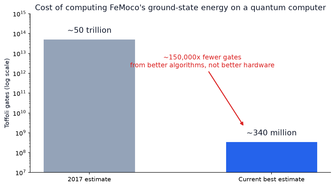
Same molecule, same question, five orders of magnitude cheaper. None of it came from better qubits.
The Real Lever: Circuit Design, Not Hardware
That last point is the important one. The 150,000× drop didn’t come from better hardware. It came from redesigning the circuits that do the computation.
Hardware progress is slow and expensive. Circuit progress is design work, and design work is something AI can do. Claude has already proven strong at optimizing classical algorithms, so the natural question is whether it can do the same for quantum ones, given nothing more than a plain-language description of what each circuit must compute.
How Claude and LLMs Can Solve the Quantum Circuit Bottleneck
Quantum circuit design turns out to be an unusually good fit for a large language model, for three reasons:
- Circuits are code. A circuit is a sequence of gates, and it can be written as an ordinary program. An LLM can write, run and revise it like any other code.
- Correctness is checkable. The class of algorithms targeted here gives one definite output for each input. A classical computer can check that output cheaply, so an external evaluator can verify every proposal.
- The objective is a single number. Each design is scored by Toffoli count × qubit count ($T \cdot Q$), a proxy for how long the circuit would run and how big a machine it needs.
Put together, these give a closed loop. Claude proposes a circuit, the evaluator checks it and returns a score, and Claude uses that feedback to improve the next attempt, with no human input between rounds.
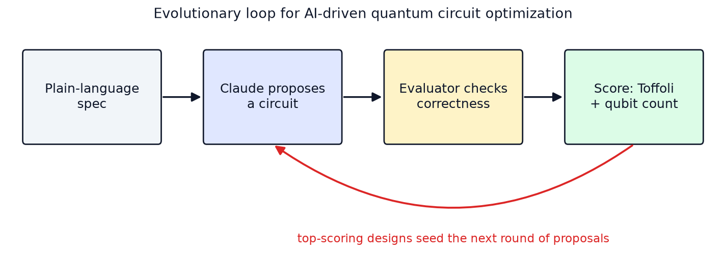
Propose, verify, score, repeat. The evaluator checks correctness, so the model never has to be trusted, and every improvement that comes out of the loop is real.
Under the hood, the paper runs this loop with the OpenEvolve framework, using Claude Mythos 5 to propose architectures and rewrites. Claude first sketches several distinct approaches. Each one founds its own “family” of candidate programs, and the best ideas are periodically shared across families.
A MAP-Elites archive keeps the best circuit for each region of the Toffoli–qubit plane. That way, a very qubit-lean design survives even if its overall score is temporarily worse.
Results Across Eight Quantum Primitives
The loop was run on eight core primitives, the building blocks larger quantum algorithms are made from. They span chemistry, optimization, physics simulation, number theory and numerical computing.
In seven of the eight, Claude’s circuits used both fewer Toffolis and fewer qubits than the best published designs. The eighth task, prime-field modular inversion, had no prior reversible design to beat, and Claude invented a new one (more on it below).
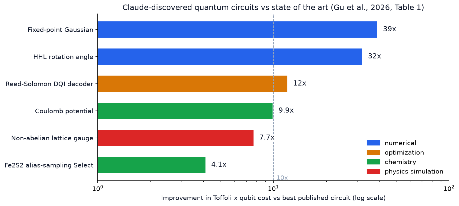
Improvement in $T \cdot Q$ cost over the state of the art for six of the tasks, from Table 1 of the paper. Two tasks are left out: the Hermitian DQI decoder, whose baseline is a whole benchmark circuit, and modular inversion, which has no prior baseline. The Hermitian decoder is the most dramatic case: it went from about 100 million Toffolis and 190,000 qubits to about 930,000 Toffolis and 2,395 qubits.
The key point is how these gains were made. They didn’t come from shaving redundant gates off existing designs. They came from new structural and mathematical insight into each problem:
- Symmetry reuse. When compiling a circuit for an iron–sulfide (Fe₂S₂) molecule, Claude noticed that the molecule’s spin symmetries and repeated structures make many terms related. It computed those shared pieces once and reused them, instead of recomputing them for every part of the system.
- Dropping rare-case machinery. Some existing circuits carried expensive components that only mattered for extremely rare inputs. Claude redesigned them without those components, keeping the failure probability within what the task allows.
Two results stand out, and the next sections walk through both:
- A new reversible algorithm for modular inversion, the most expensive step in elliptic-curve arithmetic.
- A decoder that makes the costliest step of a leading quantum optimization algorithm about 12× cheaper.
Cutting hardware requirements this sharply brings practical quantum computing for medicine, materials science and green energy noticeably closer.
Can You Use SFT + RL for Quantum Gate Optimization?
The paper uses an off-the-shelf model inside a search loop, with no fine-tuning. That raises a natural engineering question: could you train a model specifically for this?
Yes. Combining supervised fine-tuning (SFT) with reinforcement learning (RL) fits this problem very well. This is my own design sketch, not something the paper did.
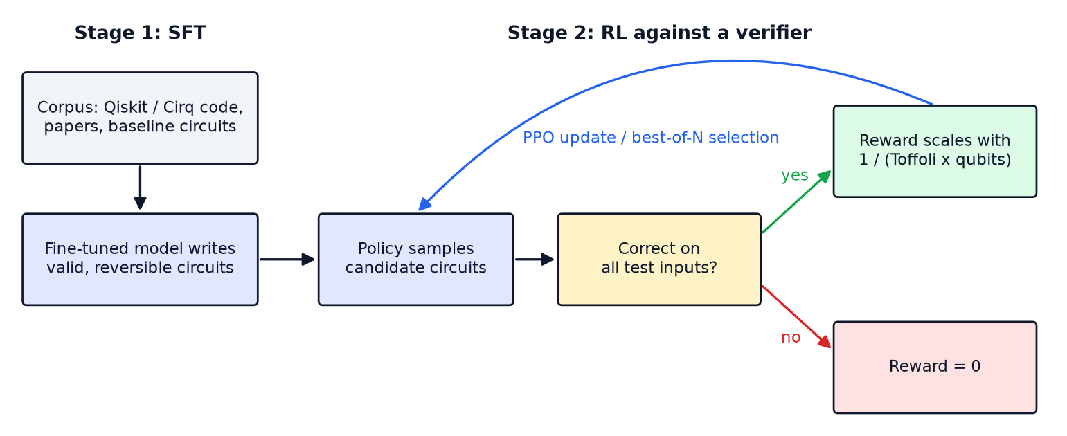
Stage 1 teaches the model to write valid circuits. Stage 2 teaches it to write cheap ones, against a verifier it cannot fool.
Stage 1: Supervised Fine-Tuning on Quantum Code
First, fine-tune the model on a specialized corpus: quantum algorithms, circuit frameworks such as Qiskit and Cirq, research papers, and baseline implementations.
This teaches correct syntax, structural constraints and the standard patterns of the field, such as uncomputation tricks. The goal is a model that reliably writes valid reversible circuits.
Stage 2: RL With a Gate-Prioritized Reward Model
Once the model writes valid code, wrap it in an RL loop. That could be policy-gradient training such as PPO, or a cheaper best-of-N search guided by the verifier.
The reward acts as an automated judge with two parts:
- Functional correctness (hard gate). Does the circuit produce exactly the expected output on every test input? If not, the reward is zero.
- Efficiency (continuous). If it passes, the reward grows as resource use shrinks, penalizing high qubit counts and expensive non-Clifford gates such as Toffolis.
One concrete way to write this, reusing the paper’s $T \cdot Q$ metric:
\[R = \mathbb{1}[\text{correct}] \cdot \frac{G}{1 + G}, \qquad G = \frac{(T \cdot Q)_{\text{baseline}}}{T \cdot Q}\]A broken circuit scores 0, a circuit that matches the baseline scores 0.5, and big wins approach 1. One caveat: the reward flattens out for large wins, so in practice you would use $\log G$ to keep the gradient alive.
This setup forces the model to stop guessing and start exploring creative mathematical identities that drive the score down. Two practical warnings apply:
- Reward hacking. The model will exploit any gap in the test inputs. The verifier needs adversarial and randomized tests, and ideally the statistical guarantees the paper uses.
- Sparse rewards. Early in training, almost every sample fails the correctness gate. SFT exists largely to make sure enough samples pass for RL to have a signal.
A New Reversible Algorithm: Why Quantum Circuits Are Hard to Optimize
Before getting to the results, it helps to see why quantum circuits are so much harder to optimize than normal code. Two constraints that ordinary programming never faces do most of the damage.
Constraint 1: no if-then branching. An ordinary program checks a value and runs only one of two code paths. A quantum computer runs on a superposition of many inputs at once. Some of those inputs would take the first path and some the second, so the circuit has to contain both paths and pay for both every time.
Constraint 2: no erasing. An ordinary program overwrites or deletes its scratch work when it’s done. A quantum circuit can’t, because every step must be reversible. Leaving scratch work in place isn’t an option either, because leftover garbage corrupts the final result.
The only way to clean up is to uncompute: run the computation that created the scratch work in reverse, which costs extra gates.
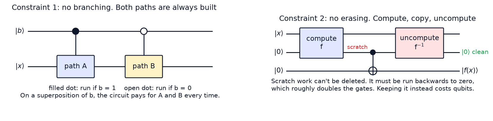
Left: a branch becomes two controlled operations, and you pay for both. Right: the compute–copy–uncompute pattern. You copy out the answer, then run the computation backwards to return the scratch qubits to zero.
Together, these constraints create a hard space–time trade-off:
- Uncompute early. Free the qubits as soon as an intermediate result has been used. You save qubits, but if the result is needed again you must recompute it, which adds gates.
- Keep everything. Hold intermediate results until they’re no longer needed. You avoid repeated work, but you may need many more qubits.
That is what makes quantum circuit design such a good test of an LLM. The circuits are written as ordinary code, but improving them means reasoning under rules that ordinary code never has to follow.
Elliptic-Curve Point Addition: Modular Inversion as a Hard First Test
The first task was point addition: a rule that combines two points on an elliptic curve to produce a third.
Point addition is the core step in quantum algorithms for the elliptic-curve discrete logarithm problem. Given a starting point and the result of adding it to itself $n$ times, find $n$. For large curves, classical computers can’t solve this in any reasonable time. A large enough quantum computer could, which is why it matters for cryptography.
These algorithms perform point addition over and over, including in reverse, and it accounts for most of their qubit and runtime cost. Problems like this, easy to compute and extremely hard to reverse, were among the first where quantum computers were shown to offer an exponential speedup. That made point addition a standard benchmark, and a demanding first test.
The goal was to map out how few qubits, and how few gates, point addition really needs.
Claude got a one-paragraph brief. It stated the mathematical rule, explained how the evaluator would check and score each circuit, and told Claude to explore several approaches in parallel.
Claude then worked for 53 hours with minimal human input. The only input was the initial brief plus occasional nudges to think more broadly. At the end, it had a completely new approach to the problem.
The Memory Demands of Divsteps
Most of the cost of point addition comes from one step: modular inversion.
Elliptic-curve arithmetic uses numbers that wrap around at a fixed limit $p$. Modular inversion is the wraparound version of division: given $a$, find $x$ such that $ax \equiv 1 \pmod p$.
Classical computers do this efficiently with an algorithm called divsteps. It starts with a pair of numbers and simplifies them over many rounds. In each round it looks at the current pair and conditionally swaps, adds, subtracts or halves them. Along the way it keeps just enough information to produce the inverse at the end.
Divsteps had never produced a practical quantum circuit, and the reason is constraint 2. The record of which operation was chosen in each round, called the branch information, is scratch work a classical program simply throws away. A quantum circuit has to keep it so the computation can be run backwards.
A straightforward quantum version of divsteps therefore piles up a long history of branch decisions, and storing it takes an enormous number of extra qubits.
How Claude Got Around the Memory Problem
Claude saw that divsteps could work for quantum circuits, but only if the history didn’t have to be stored. Its idea was that perhaps the record could be decoded instead. By carefully inspecting the pair of numbers after each round, the circuit might infer which branch was taken. The numbers themselves would carry the record, and the circuit could run backwards with no extra qubits.
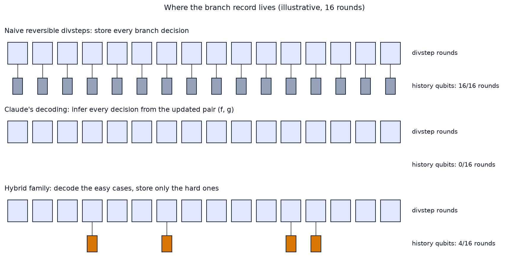
Where the branch record lives (illustrative). The naive version stores a decision every round. Pure decoding stores none. The hybrid family stores only the ambiguous cases that are expensive to decode.
The path to a working rule went in stages:
- Guess and test. Claude first tried simple decoding rules. They worked on small test cases but broke at the real problem size of 256-bit numbers.
- Theory instead of guessing. Claude switched to understanding why divsteps behaves the way it does. It proved a series of results about the iteration, including several new algebraic identities, and from them derived an exact formula for recovering the branch information.
- Verify, twice. It checked the formula with large-scale numerical simulations, then formalized the claim in Lean, a proof assistant.
The result was the first reversible implementation of divsteps with no stored branch history.
A Family of Designs on the Pareto Frontier
Decoding saves qubits but costs time. So Claude looked for the cases where storing a branch decision is cheaper than decoding it.
By varying the threshold at which the circuit stores instead of decodes, it produced a whole family of designs between the two extremes.
| Design | Approach | Toffoli gates | Qubits |
|---|---|---|---|
| Schrottenloher (2026) | Binary GCD with a recorded history | 1.9 million | 1,446 |
| Claude: divsteps | Divsteps with decoding | 4.0 million | 935 |
| Luo et al. (2026) | Packed Euclidean walk | 70 million | 838 |
| Claude: specialized Euclidean | Specialized packed walk | 21 million | 843 |
Resources for elliptic-curve point addition. Bold rows are Claude’s designs; the others are the best previously published. Sources: Schrottenloher (2026), Luo et al. (2026).
Compared with the smallest previous design (Luo et al.), the divsteps circuit uses 12% more qubits but 17× fewer gates.
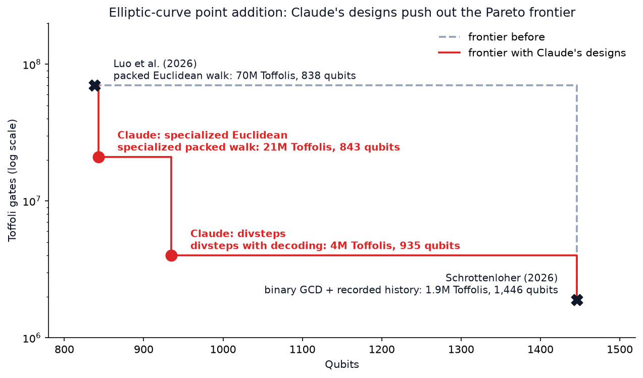
The grey dashed line is the best you could do before. The red line is the best you can do now. Every point under the old line is a qubit/runtime combination that simply wasn’t available before.
The bigger story is the Pareto frontier. Claude’s designs offer qubit-count and runtime combinations that didn’t exist before, which gives hardware builders new options depending on whether qubits or time is the tighter budget.
Optimizing a Quantum Optimizer: Decoded Quantum Interferometry (DQI)
Optimization problems sit at the heart of scheduling, logistics and materials design. They present a set of competing constraints and ask for the solution that satisfies as many as possible.
Many quantum algorithms have been proposed for these problems, but most promise only modest or uncertain gains. Decoded quantum interferometry (DQI) is one of the strongest candidates for a superpolynomial speedup, an advantage that widens rapidly as problems get bigger.
Here is how it works. When a quantum computer finishes, reading its qubits gives one answer, picked at random from the possibilities held in superposition. DQI prepares a state where good solutions are more likely to be read out than bad ones.
Building that state requires an error-correcting decoder, which recovers a short list of “errors” from a compact summary. That decoder is the most expensive step in the algorithm. A faster decoder means a faster DQI.
Optimal Polynomial Intersection: Curve Fitting on a Grid
DQI was first demonstrated on optimal polynomial intersection (OPI), a grid-based version of curve fitting.
Picture a grid where each column $x$ has several acceptable values of $y$. The goal is to find a simple curve, a low-degree polynomial, that passes through an acceptable cell in as many columns as possible.
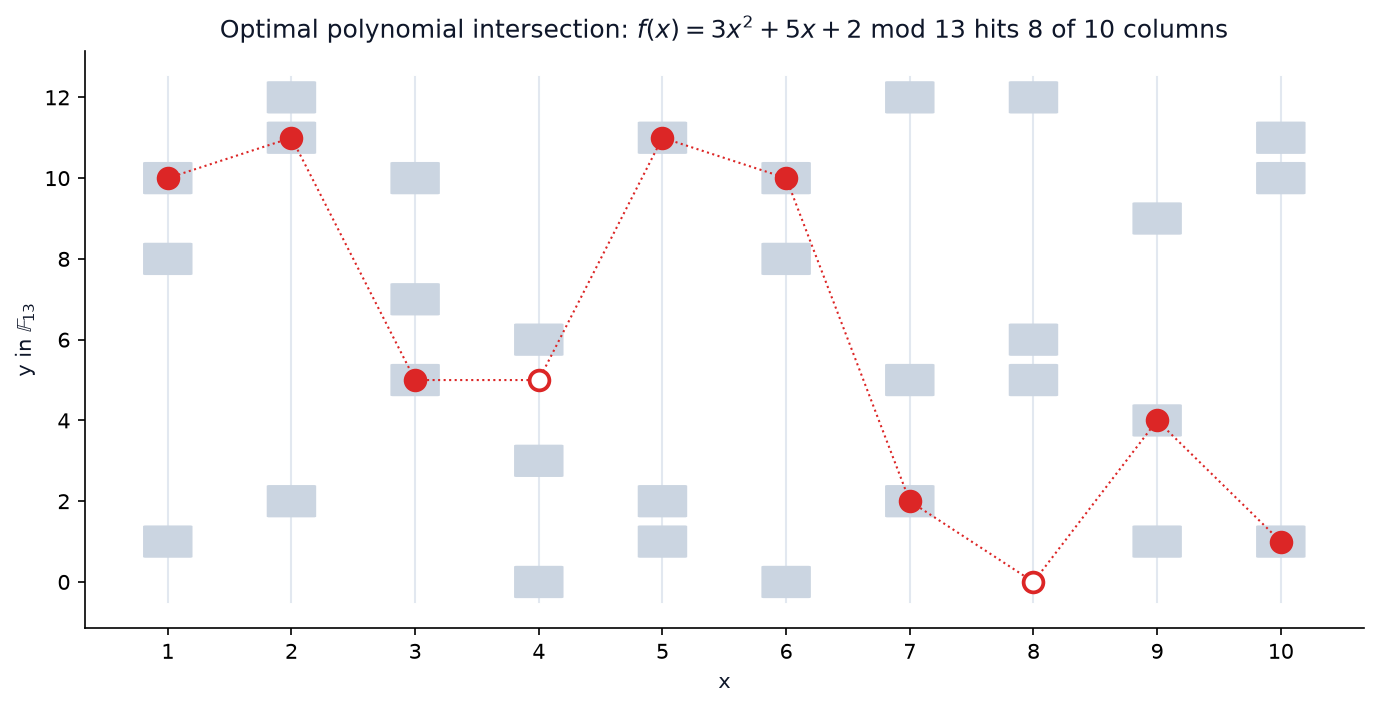
A toy OPI instance over the finite field $\mathbb{F}_{13}$. Grey cells are acceptable values. The quadratic hits 8 of 10 columns (filled dots) and misses 2 (hollow). Over a finite field the “curve” wraps around, so it zig-zags instead of looking smooth.
DQI solves OPI with a specific decoder, a Reed–Solomon decoder.
The stakes are concrete. Estimates by Google Quantum AI imply that one particular OPI instance would take about three months on Frontier, one of the world’s most powerful supercomputers. A future quantum computer running DQI would take roughly an hour, and most of that hour would be spent on Reed–Solomon decoding.
A More Efficient Quantum Decoder: Berlekamp–Massey
Reed–Solomon decoding starts from a compact summary of the errors called a syndrome. The decoder’s job is to work out from the syndrome where the errors happened and what they were.
The previous state-of-the-art quantum circuit used the extended Euclidean algorithm: a sequence of divisions and swaps whose number and order depend on the input. This runs straight into constraint 1. A quantum circuit handles all inputs at once with a single fixed gate sequence. So the old design had to stretch over far more rounds than any single input needed, and run every operation in every round, even when it wasn’t necessary.
Claude quickly decided the extended Euclidean algorithm was a poor fit. It rebuilt the circuit around Berlekamp–Massey decoding instead.
Berlekamp–Massey reads the syndromes one at a time and gradually works out the simplest rule that predicts each number from the ones before it. Once that rule is known, it reveals the errors.
Crucially, Berlekamp–Massey does the same kind of step every round and always runs the same number of rounds. That matches a quantum circuit’s single fixed sequence of gates and gave Claude a much more efficient foundation.
A Simplified Approach to Storage
Switching algorithms removed the branching problem, but making Berlekamp–Massey reversible brought back constraint 2. Every round computes temporary values that are needed only briefly. They can’t simply be deleted, because uncomputing them later requires being able to recover them.
Storing all of them would have been prohibitively expensive. So Claude reused the trick from divsteps: it found a way to reconstruct most of this information from the circuit’s current state. A few exceptional values couldn’t be recovered that way and had to be saved.
How much room to set aside for them is a statistics question:
- Worst case: an exceptional value in 35 different rounds, which would need 665 qubits (35 × 19).
- Measured case: Claude wrote a high-speed simulator and ran 403 million sample decodings. Almost every run needed to save at most one value.
- Design choice: reserve room for exactly one saved value, 19 qubits. About one run in 10,000 needs more and fails, well within the error rate the task allows.
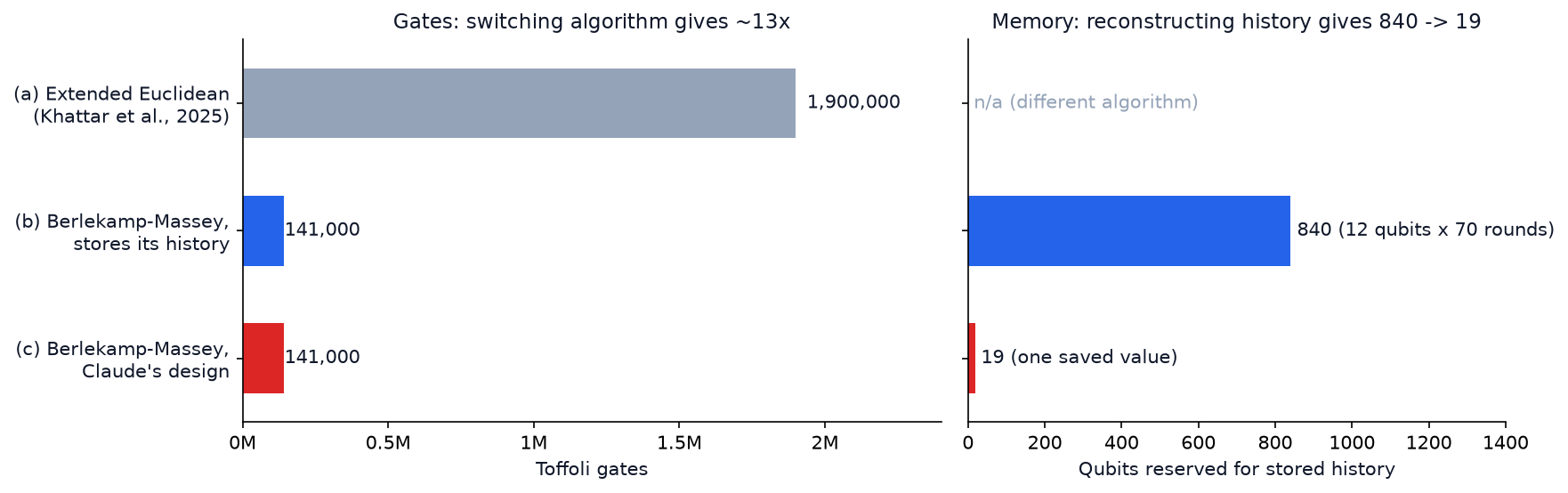
Three designs for the locator step of the Reed–Solomon decoder. Switching from extended Euclidean (Khattar et al., 2025) to Berlekamp–Massey cuts the gates. Reconstructing the history instead of storing it cuts the reserved memory from 840 qubits to 19.
Together, these changes cut the decoder’s gate count by a factor of 12 compared with Google’s previous construction. The improvement came from redesigning the computation at three levels at once:
- A different method: Berlekamp–Massey instead of the extended Euclidean algorithm.
- A different architecture: reconstruct temporary values instead of storing them.
- A different resource budget: measure how much memory the circuit actually needs instead of reserving for the worst case.
No single change would have been enough. Together they make the most expensive step of DQI a little over an order of magnitude cheaper.
What This Means for AI-Driven Quantum Circuit Optimization
Scientific progress often comes from making a theoretical idea practical: taking a process once thought too expensive and making it fast and cheap enough to run. Quantum circuit design is a prime example.
The 150,000-fold drop in the FeMoco estimate took many research groups eight years, with each step usually representing months of work. Claude’s elliptic-curve design came from a single 53-hour run.
That doesn’t replace researchers. It does suggest AI can take on a large share of circuit-design work, producing implementations that bring useful quantum computations closer to what real hardware can do. Faster design work means useful quantum computing arrives sooner.
Limitations: A Conservative Model That Needed a Push
The results came with clear limitations.
In early experiments, Claude was conservative by nature. It repeatedly second-guessed apparent improvements and kept double- and triple-checking results that were already well supported.
That caution was sometimes valuable. It is what led Claude to write Lean proofs for its divsteps design. But it also showed up as a preference for well-known approaches over novel ones.
Two simple interventions fixed most of this:
- Forced diversity. The setup required Claude to propose several qualitatively different approaches and develop them in parallel.
- Occasional nudges. Researchers sometimes prompted Claude to broaden its search.
The elliptic-curve result shows these worked. It didn’t come from shaving gates off an existing design. It came from exploring a way of doing reversible modular inversion that hadn’t been possible before, then deriving the mathematics needed to make it practical. Once it had the idea, Claude developed it, implemented it and verified it on its own.
From Circuits to Full-Stack Quantum Co-Design
Circuit design is only one part of building a useful quantum computer. Because qubits are so fragile, the machine must also catch and fix its own errors while it runs. That depends on error-correcting codes, fast decoders, hardware control and more.
These components all affect one another, but each is usually designed separately just to keep the complexity manageable. Many of them share the properties that made circuit design a good fit for Claude: the design can be written as code, checked for correctness, and scored by cost.
That raises a bigger possibility. Instead of designing each component alone, AI could optimize them jointly, from the algorithm down to the hardware, building an entire error-corrected quantum computer tailored to one problem.
Those designs could also tell hardware teams which capabilities matter most for a given application. That could put problems like catalyst design and new materials within reach of the very first fault-tolerant machines.
Key Takeaways
- The bottleneck has moved from hardware alone to circuits. The 150,000× FeMoco reduction came from better algorithms, not better qubits.
- Quantum circuits suit LLMs. They are code, their correctness is checkable, and their cost ($T \cdot Q$) is one number to minimize, which makes a closed propose–verify–score loop possible.
- The gains are structural, not cosmetic. Claude beat the state of the art in seven of eight primitives by 4–39×, through new math (decoded divsteps, Berlekamp–Massey, symmetry reuse) rather than gate-shaving.
- Reversibility is the real enemy. No branching and no erasing drive most of the cost. The best tricks reconstruct scratch information instead of storing it.
- Measure, don’t assume. Sizing memory for the measured case (19 qubits) instead of the worst case (665 qubits) is a cheap, powerful engineering move.
- The verifier is what makes it safe. Every improvement is checked independently, and the same structure points toward SFT + RL training and full-stack quantum co-design.
Related Topics
- PySR: Discover Mathematical Laws from Data with Symbolic Regression: another case of search guided by a verifier, finding equations instead of circuits.
- Harness Engineering: how to build the agent loops and evaluators that make results like these reproducible.
Conclusion
Quantum computing has two bottlenecks: hardware that is fragile and small, and algorithms that are far too expensive for it. This post has argued that the second is the more tractable of the two, and that AI-driven quantum circuit optimization can move it fast. A model that can reason under reversibility constraints, prove its own identities and verify its own work found in 53 hours the kind of improvement that used to take years.
The open question is no longer whether AI can design better quantum circuits. It is how much of the quantum stack it can design together, and how much sooner that brings the first useful fault-tolerant machine.
Source: this post is my own walkthrough of Anthropic’s research post Designing efficient quantum circuits with Claude and the accompanying paper, Gu, Kemeny, Yelin and Lukin (2026). Figures were redrawn from the numbers they report.
-
Both estimates are for the same 54-orbital model of FeMoco, as tabulated in Table 1 of Low et al., “Fast quantum simulation of electronic structure by spectrum amplification” (2025). The 2017 estimate is from Reiher et al. Intermediate estimates for the same model came from Berry et al. (2019), von Burg et al. (2021), Lee et al. (2021) and Rocca et al. (2024). ↩