SPRINT: Interleaved Planning and Parallelized Execution in Reasoning Models
A reasoning model earns its accuracy by writing a long scratchpad. It derives, checks, backtracks, and only then answers — and every token of that scratchpad is generated strictly left to right, each one conditioned on all the tokens before it. That is exactly the property that makes reasoning models slow: wall-clock time to answer scales with the length of the sequential chain, not with how much compute you own. Adding GPUs lets you run more requests; it cannot compress a chain of 20,000 dependent decoding steps into fewer steps.
But do all of those steps genuinely depend on each other? Often they do not. A model evaluating three independent cases, or checking several unrelated constraints, serializes them only because autoregressive decoding has no other gear. SPRINT is a training framework that gives the model that other gear: it teaches a reasoning model to recognize which parts of its own reasoning are independent and emit them as parallel subtasks, while keeping everything that has a real dependency in sequence.
This entry is an engineering breakdown of how you would actually build SPRINT: the inference orchestrator, the data-curation pipeline that manufactures the training set, the dependency DAG and stage-packing math, the (deliberately ordinary) training objective, and the module boundaries of a working system. The contribution is not a new optimizer or a new attention kernel — it is a data transformation plus an orchestration loop wrapped around a standard SFT run. That is the machinery we are here to reconstruct.
Scope and source discipline. The mechanism — the interleaved planner/executor loop, step extraction into plan/execution phases, the dependency DAG, the stage-packing formula, the parallelization-ratio filter, and the SFT objective — is drawn from the SPRINT paper (Biju et al., 2025). The paper evaluates on MATH-500, GPQA-Diamond, and Countdown; the quoted numbers are from those experiments. A recurring drug-discovery example is used as an applied worked example — it is our framing of the mechanism, not a domain the paper trained or tested on, and it is labelled as such wherever it appears. Where the build needs a decision the paper does not specify, it is flagged as an implementation choice.
1. The Problem: Long-Horizon Reasoning Is Serialized by Default
Start with the shape of a normal multi-step reasoning agent. A task comes in, the model reasons, it may act, it observes, it reasons again, and eventually it commits to an outcome:
Task
 ↓
LLM  ──►  Action  ──►  Environment  ──►  Observation
 ▲                                            │
 └────────────────  next reasoning step  ◄────┘
 ↓
Final Outcome
For a reasoning model the “action/observation” loop is often internal: the model’s action is to write more of its own scratchpad, and its “observation” is the context it just extended. Either way the structural fact is the same — the chain is walked one step at a time, and each step waits for the one before it.
Three properties of long-horizon reasoning turn into the pain SPRINT attacks:
- Longer traces reason better. Letting a model write more is one of the most reliable ways to raise accuracy on hard problems. This is the entire premise of reasoning fine-tuning, so we cannot simply make traces shorter.
- Longer traces cost more sequential decoding. Every extra token of the scratchpad is another forward pass that cannot overlap with any other. Latency is paid in critical-path length.
- Much of that serialization is an artifact. Independent subtasks — three cases to evaluate, five candidates to screen — get forced into a single chain purely because generation is left-to-right, not because the problem requires it.
The two existing families of inference-time scaling each fix one half and break the other:
- Sequential scaling (the DeepSeek-R1 / o1 line) coordinates perfectly — every step sees all prior work — but serializes everything, so accuracy is bought with critical-path length.
- Parallel scaling (repeated sampling, self-consistency, best-of-N) overlaps beautifully in wall-clock time, but the paths are uncoordinated: each re-derives the same facts from scratch, so N paths cost N× compute and rarely deliver N× reasoning.
Structured methods like Tree-of-Thoughts and Graph-of-Thoughts sit in between, but they require a predefined, hand-designed search structure — the branching factor and evaluation function are properties of the harness, decided per task up front, not something the model discovers about the problem it was handed.
flowchart TB
    subgraph SEQ["Sequential reasoning (LRM): coordinated but serial"]
        direction LR
        s1["Step 1"] --> s2["Step 2"] --> s3["Step 3"] --> s4["Step 4"] --> sa["Answer"]
    end
    subgraph PAR["Parallel sampling: overlapped but uncoordinated"]
        direction LR
        q(("Question")) --> pa["Path A (whole solution)"]
        q --> pb["Path B (whole solution)"]
        q --> pc["Path C (whole solution)"]
        pa --> vote["Vote / pick"]
        pb --> vote
        pc --> vote
    end
    NOTE["Gap: nothing dynamically combines real dependencies<br/>with parallel execution INSIDE one trajectory"]
    SEQ --> NOTE
    PAR --> NOTE

    style SEQ fill:#fde2e4,stroke:#e5677b
    style PAR fill:#fef9c3,stroke:#eab308
    style NOTE fill:#e0e7ff,stroke:#6366f1
Sequential methods coordinate perfectly but serialize everything; parallel methods overlap but coordinate poorly. The open question SPRINT answers: can a model, per problem, do both — branch where reasoning is independent, stay sequential where it isn’t?
The motivating question is therefore narrow and precise:
Do all reasoning steps actually need to happen sequentially — and can a model be trained to tell which ones don’t?
2. SPRINT: The Core Idea
Intuitively: SPRINT trains a reasoning model to work like a competent team lead instead of a lone worker. Faced with a problem, it first plans — reasons about what needs doing next. When it notices that several subtasks don’t depend on one another, it doesn’t grind through them one by one; it writes them down as separate assignments, hands them to a pool of workers who run them at the same time, waits for the results, folds them back into its notes, and plans the next move. Where a step genuinely needs an earlier result, it waits — exactly as a serial reasoner would.
In the authors’ framing:
SPRINT trains reasoning language models to dynamically identify and exploit parallelization opportunities during inference, achieving the accuracy of reasoning models while significantly reducing the number of sequential tokens needed to solve complex tasks.
Two words carry the weight. Trains — this lives in the weights, not in a prompt template or an external scaffold around a frozen model. Dynamically — the decomposition is produced per problem, mid-trajectory, which is precisely what the fixed structures of Tree-/Graph-of-Thoughts cannot do.
So a SPRINT trajectory interleaves two regimes:
- Sequential planning — the model reasons and decides what to do next, respecting real dependencies.
- Parallel execution — subtasks it has judged independent are dispatched and generated concurrently.
Mechanically, inference is a loop of stages. Each stage has three phases (this is the paper’s Figure 1):
flowchart LR
Q(["Query"]) --> P["Planner<br/>(fine-tuned LRM)"]
P -->|"emits <Plan_i> with<br/><prompt_i.1..j>"| DISP{"Independent<br/>subtasks?"}
DISP -->|yes| E1["Executor 1"]
DISP -->|yes| E2["Executor 2"]
DISP -->|yes| E3["Executor 3"]
E1 --> SYNC["Sync:<br/><execution_i.j> back<br/>into running context"]
E2 --> SYNC
E3 --> SYNC
SYNC --> RC[("Running context")]
RC --> P
P -->|"no more work"| ANS(["Final Answer"])
style Q fill:#fef9c3,stroke:#eab308
style P fill:#dbeafe,stroke:#3b82f6
style SYNC fill:#e0e7ff,stroke:#6366f1
style RC fill:#fde68a,stroke:#d97706
style ANS fill:#dcfce7,stroke:#22c55e
High-level SPRINT inference loop. Planner → parallel executors → sync → planner, repeating until the planner produces the final answer. The planner and every executor are the same fine-tuned model playing different roles.
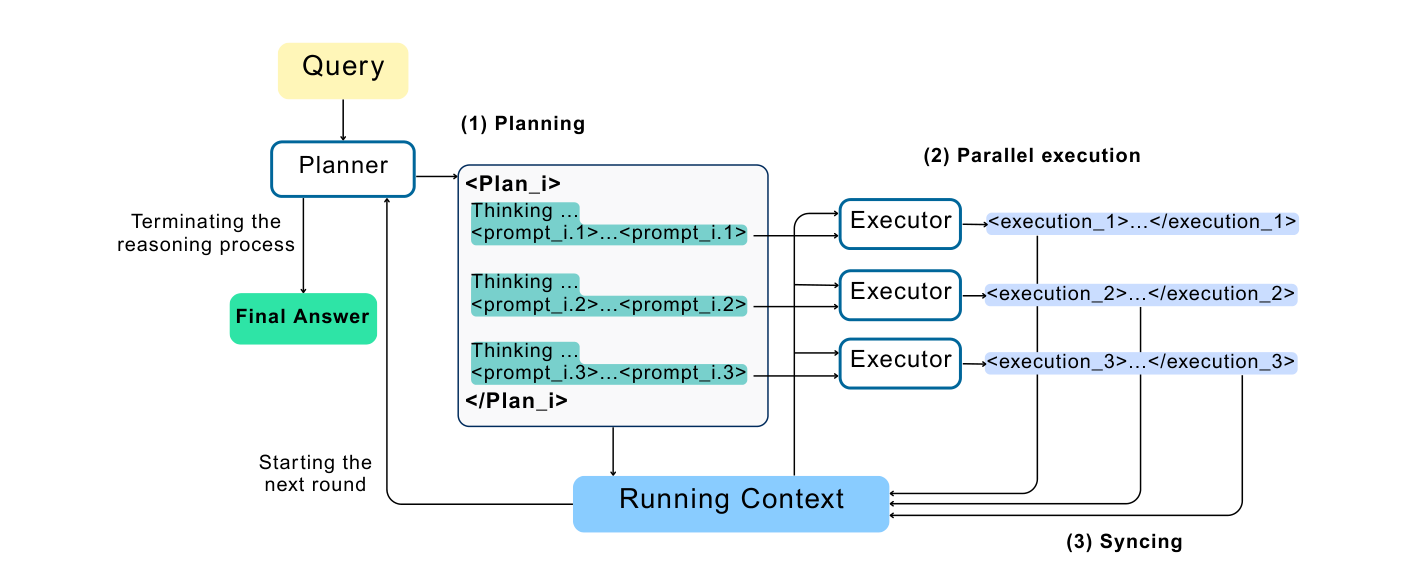
Figure 1 (SPRINT paper). One inference stage, three phases: (1) Planning — the planner reads the cumulative context and emits a <Plan_i> with one or more <prompt_i.j> subtasks (or terminates with the final answer). (2) Parallel execution — a pool of executors runs those prompts concurrently. (3) Syncing — the <execution_i.j> outputs are appended back into the running context, in prompt order, and control returns to the planner.
How it differs from conventional multi-step RL / reasoning:
| Axis | Conventional serial LRM | SPRINT |
|---|---|---|
| Training method | RL or SFT on serial traces | SFT on restructured serial traces |
| Trajectory shape | one long left-to-right chain | interleaved sequential + parallel stages |
| Who decides the structure | decoding order (implicit) | the model, per problem, at inference |
| What is optimized | quality/length of the chain | reproducing a parallelizable layout |
| Latency lever | none (chain length is fixed) | shorten the critical path, not total work |
Why this helps training and inference: the parallel branches within a stage are independent, so an error in one cannot contaminate the others — the planner reconciles them afterward, which supplies a self-consistency-like diversity benefit and isolates errors. And because independent work moves off the critical path, the longest dependency chain the model must walk gets shorter — which is the quantity that determines latency.
3. SPRINT Architecture
SPRINT has two halves that must be kept distinct in your head, because they run at different times and use different machinery:
The curation pipeline builds the training data (offline, one time). The inference framework executes the learned behavior (online, per query). Fine-tuning connects them.
flowchart TB
subgraph CUR["Data curation (offline) — teacher model + code"]
RAW[("Raw DeepSeek-R1<br/>reasoning trajectories")] --> FILT0["Correctness filter<br/>(verifiable answers)"]
FILT0 --> EXT["Step extraction<br/>GPT-4o → (Pᵢ, Eᵢ)"]
EXT --> DAG["Dependency DAG<br/>GPT-4o-mini → D, G=(S,D)"]
DAG --> PACK["Stage packing<br/>σ(Sᵢ) — plain code"]
PACK --> RATIO["Parallelization-ratio filter<br/>|S| / #stages ≥ 1.5"]
RATIO --> REF["Reformat into<br/><Plan_i>/<prompt>/<execution>"]
REF --> DS[("~1,700 structured<br/>SFT examples")]
end
DS --> SFT["Supervised fine-tuning<br/>(next-token loss)"]
SFT --> MODEL["SPRINT-trained LRM"]
subgraph INF["Inference framework (online) — one model, two roles"]
MODEL --> PL["Planner role"]
PL --> ORCH["Orchestrator:<br/>parse prompts, dispatch,<br/>synchronize"]
ORCH --> EXP["Executor pool<br/>(concurrent)"]
EXP --> CTX[("Running context")]
CTX --> PL
PL --> OUT(["Final answer"])
end
style CUR fill:#eef2ff,stroke:#6366f1
style INF fill:#f0fdf4,stroke:#22c55e
style DS fill:#fef9c3,stroke:#eab308
style RAW fill:#fde2e4,stroke:#e5677b
System boundaries. The teacher model (GPT-4o / GPT-4o-mini) and the packing code appear only in curation — never at inference. At serve time there is one model, an orchestrator, and a context store. Fine-tuning is the single bridge.
Mapping the generic agent-RL skeleton onto SPRINT’s actual components (using the paper’s terminology):
| Generic stage | SPRINT component | Where |
|---|---|---|
| Task dataset | MATH training queries (→ R1 trajectories) | curation input |
| Agent / policy model | DeepSeek-R1-Distill-Qwen-7B (the LRM being trained) | training/inference |
| Agent runtime | the interleaved planner/executor orchestrator | inference |
| Reasoning / planning | the planner role emitting <Plan_i> |
inference |
| Tool / environment | (none in-paper — executors generate tokens; tool use is future work) | — |
| Trajectory collection | DeepSeek-R1 produces raw reasoning traces | curation input |
| SPRINT processing | step extraction → DAG → packing → filter/reformat | curation |
| Training examples | ~1,700 structured plan/execution sequences | curation output |
| RL / policy optimization | plain SFT (no reward, no policy gradient) | training |
| Updated policy | the SPRINT-trained LRM | output |
The one row worth pausing on is tool / environment: the paper’s executors do not call tools — they generate a chain-of-thought to accomplish a subtask. Parallel tool use (docking APIs, retrievers, ADMET predictors) is explicitly flagged as future work. If you build SPRINT with real tools, that is an extension, not the paper’s system.
4. Trajectory Generation: Where the Raw Material Comes From
SPRINT does not collect “parallel reasoning” data — no teacher is ever prompted to reason in parallel. It starts from ordinary long reasoning trajectories and converts them into a parallel-aware format. So “trajectory generation” here means: run a strong reasoning model on a task and record its complete serial scratchpad.
Task (a MATH problem Q)
 ↓
DeepSeek-R1 reasons (left-to-right chain-of-thought)
 ↓
line 1 … line 2 … "let's verify" … line 200: final answer
 ↓
Raw reasoning trajectory τ  (one long serial trace)
Formally, the paper works with the trace as a sequence of discrete reasoning steps rather than an RL state–action tuple. A trajectory $\tau$ for query $Q$ decomposes into
\[S = \{S_1, S_2, \ldots, S_n\}, \qquad S_i = (P_i, E_i)\]where each step $S_i$ is split into a planning phase $P_i$ (the model deciding what to do — reframing the problem, naming a subtask, noting a constraint) and an execution phase $E_i$ (actually carrying that subtask out — the calculation or derivation). Some steps are plan-only: they have $E_i = \emptyset$ because there is nothing substantial to farm out.
What must be captured per step, and why:
- $P_i$ — the plan text. This is the part the planner will learn to emit and, when it names independent work, to dispatch.
- $E_i$ — the execution text (or $\emptyset$). This is the part an executor will learn to produce given a prompt. Empty for plan-only steps.
- Order index $i$. Dependencies can only point backward ($i < j$), so original order is needed to build a valid DAG.
In their experiment the scale is modest and worth internalizing: 6,000 DeepSeek-R1 trajectories on the MATH training set, correctness-filtered and curated down to ~1,700 structured examples, used to fine-tune DeepSeek-R1-Distill-Qwen-7B.
Honest note on the word “trajectory.” SWiRL’s trajectory is an environment-interaction sequence (tool call → observation → next action). SPRINT’s raw trajectory is a pure reasoning trace with no environment. The
state → action → observationloop from classical agent RL is not what SPRINT trains on — a point that matters when comparing the two methods (§14).
5. The SPRINT Data-Construction Process
This is the heart of the method. Raw serial reasoning goes in; a structured, parallelizable training example comes out. The pipeline (paper’s Figure 2) is four stages after correctness filtering:
Raw R1 trajectory
   ↓  (1) step extraction        — GPT-4o
Steps Sᵢ = (Pᵢ, Eᵢ), some plan-only
   ↓  (2) dependency DAG         — GPT-4o-mini
G = (S, D)
   ↓  (3) stage packing          — plain code (σ formula)
Stages L⁽¹⁾, L⁽²⁾, …
   ↓  (4) filter + reformat      — ratio ≥ 1.5, tag layout
Structured SFT example
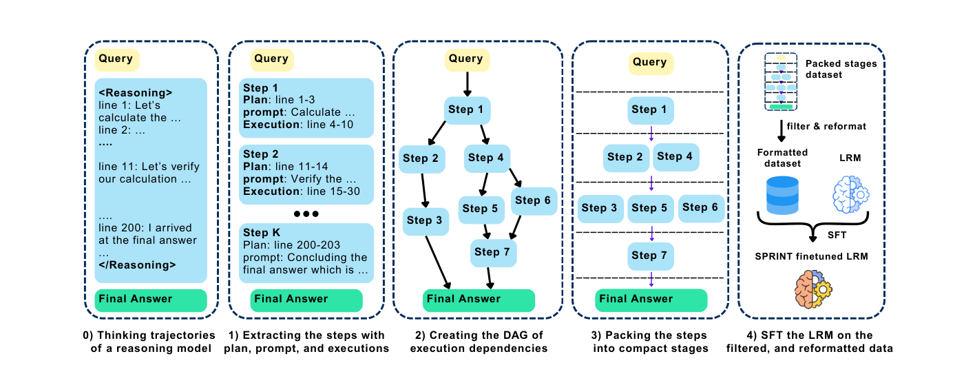
Figure 2 (SPRINT paper). The curation pipeline. Notice the transformation in panels (2)→(3): the DAG’s independent nodes (e.g. steps 2 and 4, or 3, 5 and 6) collapse into the same stage, while dependent nodes stay in separate rows. The parallel structure is read off the dependency graph, never off textual order.
Let’s walk it on a concrete multi-step example. Take a math-style trace (the paper’s domain), then we mirror it with the drug-discovery application.
Step 1 → Set up the problem; identify it needs three independent sub-quantities.
Step 2 → Compute quantity A.
Step 3 → Compute quantity B.
Step 4 → Compute quantity C.
Step 5 → Combine A, B, C into the result.
Stage 1 — step extraction (GPT-4o)
An LLM reads the raw trace and splits each step into plan and execution:
Step 2
  Plan (P₂):      "Compute quantity A."
  Execution (E₂): [the arithmetic / derivation for A]
Two curation rules matter here. First, plan-only steps (deciding, reframing) carry no executor call — they stay entirely on the planner side. Second, very short executions are merged back into their plan, becoming plan-only, so the planner handles trivial work itself instead of paying dispatch overhead to farm out one line.
Stage 2 — dependency DAG (GPT-4o-mini)
A separate, smaller model is asked which steps depend on which. Dependencies are the edge set
\[D = \{(S_i, S_j) \mid S_j \text{ depends on } S_i,\; i < j,\; S_i, S_j \in S\}\]forming a directed acyclic graph $G = (S, D)$. For our example:
flowchart TD
    S1["S₁ setup"] --> S2["S₂ compute A"]
    S1 --> S3["S₃ compute B"]
    S1 --> S4["S₄ compute C"]
    S2 --> S5["S₅ combine"]
    S3 --> S5
    S4 --> S5

    style S1 fill:#dbeafe,stroke:#3b82f6
    style S2 fill:#dcfce7,stroke:#22c55e
    style S3 fill:#dcfce7,stroke:#22c55e
    style S4 fill:#dcfce7,stroke:#22c55e
    style S5 fill:#fde68a,stroke:#d97706
The load-bearing discipline: you establish dependencies first, and parallelism falls out as a consequence. Textual adjacency is not independence — three consecutive steps could equally be a chain where each refines the last. S₂/S₃/S₄ are parallel only because the DAG has no edges among them.
Stage 3 — pack the DAG into stages
Now group steps into stages such that everything in a stage can be planned together and executed concurrently. The paper defines a stage number $\sigma(S_i)$ for each step $S_i = (P_i, E_i)$:
\[\sigma(S_i) = \begin{cases} 1, & \text{if } S_i \text{ has no parents} \\[4pt] \displaystyle\max_{S_p \in \text{Parents}(S_i)} \big(\sigma(S_p) + \mathbb{1}(E_p \neq \emptyset)\big), & \text{otherwise} \end{cases}\]Read it carefully — the indicator $\mathbb{1}(E_p \neq \emptyset)$ is the clever part:
- A step with no parents lands in stage 1.
- Otherwise its stage is the max over its parents of the parent’s stage plus one — but only if the parent actually executed something. If a parent $S_p$ is plan-only ($E_p = \emptyset$), you do not advance the stage. A plan-only parent produces no executor output to wait on, so its child can safely sit in the same stage. This is the “plan-only parent” optimization: it both guarantees the child has the context it needs and packs the schedule tighter.
The set of steps at stage $k$ is
\[\mathcal{L}^{(k)} = \{S_i \in S \mid \sigma(S_i) = k\}\]Within a stage, the combined plan concatenates the plans (in original order) and the execution set collects every non-empty execution:
\[\mathcal{P}^{(k)} = \text{concat}\big(P_i \mid S_i \in \mathcal{L}^{(k)}\big), \qquad \mathcal{E}^{(k)} = \{E_i \mid S_i \in \mathcal{L}^{(k)},\; E_i \neq \emptyset\}\]Our five steps collapse from a chain of length 5 into a critical path of length 3:
Stage 1:  S₁                       (setup)
Stage 2:  S₂ , S₃ , S₄   ← parallel (compute A, B, C together)
Stage 3:  S₅                       (combine)
That compression — five serial steps into a three-deep critical path — is the entire source of SPRINT’s latency win. No work was removed; work was moved off the critical path.
Stage 4 — filter and reformat
Not every trajectory is worth keeping. The parallelization ratio
\[\rho = \frac{\#\text{reasoning steps}}{\#\text{stages}} = \frac{|S|}{K}\]must be at least 1.5, or the example is discarded. A pure chain scores $\rho = 1.0$ and teaches nothing about parallelism; our example scores $5/3 \approx 1.67$ and survives. (The paper’s seven-step / four-stage illustration scores $1.75$.)
Survivors are reformatted into the tagged layout the model will learn to produce:
<query> … </query>

<Plan_1> Set up the problem and identify the sub-quantities. </Plan_1>
<execution_1.1> … </execution_1.1>

<Plan_2>
  <prompt_2.1> Compute quantity A. </prompt_2.1>
  <prompt_2.2> Compute quantity B. </prompt_2.2>
  <prompt_2.3> Compute quantity C. </prompt_2.3>
</Plan_2>
<execution_2.1> [result A] </execution_2.1>
<execution_2.2> [result B] </execution_2.2>
<execution_2.3> [result C] </execution_2.3>

<Plan_3> Combine A, B, C into the final result. </Plan_3>
<execution_3.1> [combination] </execution_3.1>

<Final Answer> … </Final Answer>
The whole sequence is the training target — the model must learn when to open a plan block, how many prompts to put in it, and when to stop and wait for results.
flowchart LR
    RAW[("Raw serial trace")] --> A["1· Extract steps<br/>(Pᵢ, Eᵢ)"]
    A --> B["2· Infer dependencies<br/>D, DAG G=(S,D)"]
    B --> C["3· Pack via σ(Sᵢ)<br/>into stages L⁽ᵏ⁾"]
    C --> D{"ρ = |S|/K ≥ 1.5 ?"}
    D -->|no| DROP["Discard"]
    D -->|yes| E["4· Reformat into<br/>Plan/prompt/execution tags"]
    E --> OUT[("SFT example")]

    style RAW fill:#fde2e4,stroke:#e5677b
    style B fill:#dbeafe,stroke:#3b82f6
    style C fill:#e0e7ff,stroke:#6366f1
    style DROP fill:#fee2e2,stroke:#ef4444
    style OUT fill:#dcfce7,stroke:#22c55e
Applied mirror (drug discovery, our framing). The identical pipeline on “given protein P and candidates A, B, C, find the strongest binder”: setup + binding-pocket identification (Stage 1) → evaluate A, B, C against the pocket in parallel (Stage 2) → compare (Stage 3) → investigate the winner (Stage 4). The DAG is what encodes “A, B, C are independent, but comparing them must wait for all three.” Same mechanism, scientific workload.
6. Step-Wise / Multi-Step Learning: What the Model Actually Internalizes
Make the relationships explicit, because “parallel reasoning” is easy to over-read:
| Concept | In SPRINT |
|---|---|
| Task | the query $Q$ |
| Trajectory | the full stage sequence: $Q \to (\mathcal{P}^{(1)}, \mathcal{E}^{(1)}) \to \cdots \to$ answer |
| Intermediate state | the running context: query + all prior plans + all prior executions |
| Action (planner) | emit <Plan_i> containing one or more <prompt_i.j> |
| Action (executor) | produce <execution_i.j> for one prompt, given the context snapshot |
| Feedback | synchronization: executor outputs appended back in prompt order |
| Training unit | the stage — a combined plan plus its concurrent executions |
The training unit is the stage, and that is the whole design move. A stage bundles a plan (which may assert “these $j$ subtasks are independent”) with the executions that plan spawned. A plan block holding three sibling prompts is a learned assertion that those three subtasks can run concurrently — there is no separate PARALLELIZE_THIS label anywhere. The supervision signal is format. Ordinary SFT on the tagged layout teaches the branching behavior.
flowchart TB
    subgraph BEFORE["Serial trace (what the teacher produced)"]
        direction LR
        b1["S₁"] --> b2["S₂"] --> b3["S₃"] --> b4["S₄"] --> b5["S₅"]
    end
    BEFORE ==>|"dependency DAG + packing"| AFTER
    subgraph AFTER["SPRINT stages (what the student learns to emit)"]
        direction TB
        a1["Stage 1: Plan₁ + Exec₁"] --> a2["Stage 2: Plan₂ = {prompt A, B, C}<br/>Exec A ∥ Exec B ∥ Exec C"]
        a2 --> a3["Stage 3: Plan₃ + Exec₃ (combine)"]
    end

    style BEFORE fill:#fde2e4,stroke:#e5677b
    style AFTER fill:#f0fdf4,stroke:#22c55e
    style a2 fill:#dbeafe,stroke:#3b82f6
Why this representation improves long-horizon learning: because the states in the training set are drawn from real trajectories that had to go somewhere, learning to produce good local stage structure across that distribution also improves global behavior. And critically, packing is what makes the trace’s critical path short — the model isn’t just imitating text, it is imitating a text whose shape encodes parallelism. One clarification that avoids a common misread: this is one policy emitting a structured sequence, not a separate model per stage. “Planner” and “executor” are roles the single fine-tuned model plays, not distinct trained artifacts.
7. Reward / Feedback: There Is No Reward Model
This section exists mostly to prevent a wrong inference. Because SWiRL, PPO, GRPO and the rest of the RL family all revolve around a reward, it is tempting to assume SPRINT has one. It does not. SPRINT is supervised fine-tuning; there is no reward function, no advantage, no policy gradient, no reward model. Be precise about the three things that could be mistaken for a training signal:
- Verifiable correctness — used only as a data filter. Before curation, the 6,000 raw DeepSeek-R1 traces are filtered for correctness against MATH’s golden answers. This selects which traces are worth curating — it never enters the loss. It is verifiable feedback applied to data selection, not reward optimization.
- Synchronization — an inference-time information flow, not a reward. When executors finish, their
<execution_i.j>outputs are synced back into the running context in prompt order. This is how later planning “sees” earlier results — it is context assembly, not scoring. Nothing grades the executor. - The SFT target — the only training signal. The model is optimized to reproduce the curated, restructured sequence token-for-token. That target sequence is the supervision.
flowchart LR
    RAW[("6,000 raw R1 traces")] --> CF{"Correct vs<br/>golden answer?"}
    CF -->|no| X["Dropped from curation"]
    CF -->|yes| CUR["Curate → SFT target"]
    CUR --> LOSS["Next-token loss<br/>(the only signal)"]

    SYNC["Executor outputs synced<br/>into running context"] -.->|"context, NOT reward"| PLAN["Next planning step"]

    style CF fill:#fef9c3,stroke:#eab308
    style X fill:#fee2e2,stroke:#ef4444
    style LOSS fill:#dcfce7,stroke:#22c55e
    style SYNC fill:#e0e7ff,stroke:#6366f1
The correctness filter is a data gate; synchronization is inference-time context flow. Neither is a reward. If you want to see where reward-based post-training (RLHF, RLVR, PPO, GRPO, DPO) fits relative to this, that is the subject of the companion RL blog linked in §15.
8. Mathematical Formulation
SPRINT’s math is entirely in the data transformation; the learning objective is deliberately standard. Here are the equations that matter, each with its role in the pipeline.
(1) Steps and phases. Each reasoning step is a plan/execution pair:
\[S_i = (P_i, E_i), \qquad E_i = \emptyset \text{ for plan-only steps}\]Variables: $P_i$ = planning text, $E_i$ = execution text (or empty). Intuition: separates the dispatchable part (plan) from the farmable part (execution). Pipeline: output of step extraction (§5, Stage 1). Optimized: nothing yet — this is data structure.
(2) Dependency set and DAG.
\[D = \{(S_i, S_j) \mid S_j \text{ depends on } S_i,\; i<j\}, \qquad G = (S, D)\]Variables: an edge $(S_i,S_j)$ means $S_j$ needs $S_i$’s result; $i<j$ enforces acyclicity. Intuition: this is the ground truth of “what must stay sequential.” Pipeline: output of DAG creation (§5, Stage 2). Optimized: nothing — but it constrains everything downstream.
(3) Stage number (the packing rule).
\[\sigma(S_i) = \begin{cases} 1, & S_i \text{ has no parents} \\ \max\limits_{S_p \in \text{Parents}(S_i)} \big(\sigma(S_p) + \mathbb{1}(E_p \neq \emptyset)\big), & \text{otherwise} \end{cases}\]Variables: $\text{Parents}(S_i)$ = steps $S_i$ depends on; $\mathbb{1}(\cdot)$ = 1 if the parent had a real execution, else 0. Intuition: a child advances one stage past its parents only when a parent produced an execution result to wait on; a plan-only parent lets the child share its stage. Pipeline: the packing algorithm (§5, Stage 3) — plain code, not a model call. Optimized: minimizes stage count (critical-path depth) subject to dependencies.
(4) Stage contents.
\[\mathcal{L}^{(k)} = \{S_i \mid \sigma(S_i)=k\}, \quad \mathcal{P}^{(k)} = \text{concat}(P_i \mid S_i \in \mathcal{L}^{(k)}), \quad \mathcal{E}^{(k)} = \{E_i \mid S_i \in \mathcal{L}^{(k)}, E_i \neq \emptyset\}\]Intuition: everything in stage $k$ is planned together and executed concurrently. Pipeline: defines the tagged training example.
(5) Parallelization-ratio filter.
\[\rho = \frac{|S|}{K} \ge 1.5, \qquad K = \#\text{stages}\]Intuition: keep only trajectories with enough parallel structure to teach the behavior. Pipeline: the discard gate (§5, Stage 4).
(6) The training objective — standard supervised fine-tuning. Let $Y$ be the reformatted target sequence (all stage-wise plan/execution/answer tokens) for query $Q$. The model is trained by ordinary next-token cross-entropy:
\[\mathcal{L}_{\text{SFT}}(\theta) = -\sum_{t=1}^{|Y|} \log \pi_\theta\big(y_t \mid y_{<t}, Q\big)\]Variables: $\pi_\theta$ = the LRM being fine-tuned; $y_t$ = the $t$-th target token; $Q$ = query. Intuition: teacher-forced imitation of the restructured trajectory — no reward, no advantage. Pipeline: the SFT stage. Optimized: the likelihood of producing the parallelizable layout, which is precisely the behavior SPRINT unlocks.
Implementation choice (labelled). The paper states the objective as “fine-tune the LRM on the reformatted thinking patterns” and does not print a bespoke loss; the cross-entropy above is the standard SFT loss that phrasing denotes. Whether you mask loss on the query tokens, or weight plan vs. execution spans, is an ordinary SFT engineering decision the paper does not prescribe.
9. The Training Loop
Because SPRINT is offline SFT, “the training loop” splits into a one-time curation loop and a standard SFT loop. There is no online rollout-and-reward cycle.
flowchart TD
    INIT["Base LRM (R1-Distill-Qwen-7B)"] --> GEN["Generate raw traces with teacher (DeepSeek-R1) on MATH"]
    GEN --> CFILT["Correctness filter"]
    CFILT --> PROC["SPRINT processing:<br/>extract → DAG → pack"]
    PROC --> RFILT["ρ ≥ 1.5 filter + reformat"]
    RFILT --> DSET[("~1,700 structured examples")]
    DSET --> TRAIN["SFT: minimize next-token loss"]
    TRAIN --> EVAL["Evaluate:<br/>accuracy + sequential tokens"]
    EVAL --> DONE(["SPRINT-trained LRM"])

    style INIT fill:#fde2e4,stroke:#e5677b
    style PROC fill:#dbeafe,stroke:#3b82f6
    style DSET fill:#fef9c3,stroke:#eab308
    style TRAIN fill:#e0e7ff,stroke:#6366f1
    style DONE fill:#dcfce7,stroke:#22c55e
One “iteration” of the real training is just one SFT step: sample a batch of structured examples, teacher-force the target sequences, backprop the cross-entropy, update $\theta$. Nothing samples fresh rollouts; nothing scores them. Repeated iterations simply fit the model to the parallelizable layout across the ~1,700 examples until it reliably (a) emits <Plan_i> blocks, (b) puts the right number of independent <prompt>s in them, and (c) stops to wait at synchronization points.
The clean part of the experimental design: an ordinary reasoning-fine-tuned (RFT) baseline is trained on the same ~1,700 trajectories, just without restructuring. Same content, same volume, same source — only the structure of the supervision differs. That isolates the question “does restructuring for parallel execution help?” and the answer (§13) is yes.
10. Engineering Implementation
Now from algorithm to software. Organize the build around the modules the paper’s method actually requires. The curation modules run once; the runtime modules run per query.
Task Manager
Holds the query set (MATH problems for training-data generation; the live query at inference). At curation time it also owns the correctness filter that gates raw traces. Paper terms: query $Q$, correctness filtering.
Trajectory Generator (curation only)
Runs the teacher (DeepSeek-R1) to produce raw serial reasoning traces. Not needed at inference. Implementation choice: you can swap any strong reasoning model here; the paper uses R1.
SPRINT Processor (curation only)
The core module, itself three sub-stages:
def sprint_process(trace, extractor_llm, dag_llm):
    steps = extractor_llm.extract(trace)        # GPT-4o: [(P_i, E_i), ...], plan-only where E_i=None
    steps = merge_short_executions(steps)       # tiny E_i folded into P_i → plan-only
    D = dag_llm.infer_dependencies(steps)        # GPT-4o-mini: edge set {(i, j): j depends on i}
    stages = pack_stages(steps, D)               # plain code: the σ(S_i) recurrence
    if parallelization_ratio(steps, stages) < 1.5:
        return None                              # discard: not enough parallelism
    return reformat(steps, stages)               # tagged <Plan_i>/<prompt>/<execution> sequence
with the packing recurrence exactly mirroring the σ formula:
def pack_stages(steps, D):
    parents = build_parents(D)                   # parents[i] = {p : (p, i) in D}
    sigma = {}
    for i in topological_order(steps, D):        # i < j guarantees a valid order
        if not parents[i]:
            sigma[i] = 1
        else:
            sigma[i] = max(
                sigma[p] + (0 if is_plan_only(steps[p]) else 1)   # 1(E_p != ∅)
                for p in parents[i]
            )
    stages = group_by_stage(sigma)               # L^(k) = {i : sigma[i] == k}
    return stages
Note: the extractor and DAG models are prompted, not fine-tuned — they are data curators. Prompting them is not the SFT.
Training Worker
Standard SFT on the structured examples — the objective from §8. No RL infrastructure (no reward server, no rollout buffer). Paper terms: SFT of the LRM.
Agent Runtime / Orchestrator (inference)
The interleaved-execution engine. Owns the stage loop: give the planner the running context, parse the emitted <prompt_i.j> tags, dispatch them to executors, await all, sync results back in order, repeat until a final answer.
def sprint_infer(query, model, executor_pool):
    context = [query]
    while True:
        plan = model.plan(context)               # planner role: emits <Plan_i> with <prompt>s
        if plan.is_final_answer:
            return plan.answer
        prompts = plan.prompts                    # [] means plan-only → planner continues itself
        # THE PARALLEL STEP: independent subtasks run concurrently
        results = executor_pool.map(              # each executor = same model, executor role
            lambda p: model.execute(context_snapshot(context), p),
            prompts
        )
        # SYNC: append <execution_i.j> in prompt order
        context += [plan] + order_by_prompt(results)
Environment / Tool Executor
In the paper, “execution” is token generation — no external tools. The executor_pool.map above dispatches to model instances. Extension (future work, labelled): replace model.execute with real tool calls (retriever, docking API, ADMET predictor) so independent tool invocations overlap — where the latency payoff is far larger than parallelizing token generation.
Trajectory Store
Persists raw traces, extracted steps, DAGs, and packed stages during curation so the expensive teacher/curator calls are not repeated. Implementation choice: not specified by the paper; standard data-pipeline hygiene.
Evaluation System
Measures the two quantities that define success: accuracy and sequential tokens (§13). Sequential tokens require the orchestrator to record, per stage, the max executor length rather than the sum.
Hardware note (a real limitation, not a detail)
The authors are explicit: the logical parallelism SPRINT emits only becomes wall-clock speedup with an optimized serving stack — KV-cache mechanisms for concurrent branches, high-bandwidth GPU interconnect, and enough GPU slots to actually run the executors at once. They did not build that optimal system. SPRINT creates the parallel workload; a serving system still has to execute it well.
11. Data Structures
The raw trace and the structured training example are two different objects. First, what curation ingests and produces internally:
raw_trajectory = {
    "query": "Given protein P and candidates A, B, C, find the strongest binder.",
    "trace": "<Reasoning> line 1 … line 200: final answer </Reasoning>",
    "correct": True,                       # correctness filter (data gate, not reward)
}

steps = [
    {"id": 1, "plan": "Identify the binding pocket of P.", "execution": "..."},
    {"id": 2, "plan": "Evaluate candidate A vs. pocket.", "execution": "..."},
    {"id": 3, "plan": "Evaluate candidate B vs. pocket.", "execution": "..."},
    {"id": 4, "plan": "Evaluate candidate C vs. pocket.", "execution": "..."},
    {"id": 5, "plan": "Compare A, B, C.",                "execution": "..."},
]

dependencies = [(1, 2), (1, 3), (1, 4), (2, 5), (3, 5), (4, 5)]   # edge set D
stages = {1: [1], 2: [2, 3, 4], 3: [5]}                            # L^(k) after packing
Then the reformatted SFT target — a single flat token sequence with the tag layout, which is what the model is trained on end to end:
<query> Given protein P and candidates A, B, C, find the strongest binder. </query>

<Plan_1> Analyze P and identify the binding pocket.
  <prompt_1.1> Identify the pocket and key residues. </prompt_1.1>
</Plan_1>
<execution_1.1> …pocket characterized… </execution_1.1>

<Plan_2>
  <prompt_2.1> Evaluate A against the pocket. </prompt_2.1>
  <prompt_2.2> Evaluate B against the pocket. </prompt_2.2>
  <prompt_2.3> Evaluate C against the pocket. </prompt_2.3>
</Plan_2>
<execution_2.1> …A binds moderately… </execution_2.1>
<execution_2.2> …B binds weakly… </execution_2.2>
<execution_2.3> …C binds strongly… </execution_2.3>

<Plan_3> Compare A, B, C and pick the strongest. </Plan_3>
<execution_3.1> …C is strongest… </execution_3.1>

<Final Answer> Candidate C. </Final Answer>
The only fields that matter are the ones the paper defines: plan ($P_i$), execution ($E_i$, possibly empty), step order, dependency edges, and stage assignment. There is no reward field, no advantage, no value estimate — because there is no RL.
12. End-to-End Example
One complete pass, using the drug-discovery application (mechanism from the paper; workload is our framing).
flowchart TD
U(["User task:<br/>rank binders A, B, C for protein P"]) --> P1["Planner (Stage 1):<br/><Plan_1> identify pocket"]
P1 --> E1["Executor: characterize pocket"]
E1 --> S1["Sync → running context"]
S1 --> P2["Planner (Stage 2):<br/><Plan_2> = {eval A, eval B, eval C}<br/>(now independent!)"]
P2 --> EA["Executor A"]
P2 --> EB["Executor B"]
P2 --> EC["Executor C"]
EA --> S2["Sync (in prompt order)"]
EB --> S2
EC --> S2
S2 --> P3["Planner (Stage 3):<br/><Plan_3> compare A,B,C"]
P3 --> E3["Executor: comparison"]
E3 --> S3["Sync"]
S3 --> ANS(["Final Answer: C"])
style U fill:#fef9c3,stroke:#eab308
style P2 fill:#dbeafe,stroke:#3b82f6
style EA fill:#dcfce7,stroke:#22c55e
style EB fill:#dcfce7,stroke:#22c55e
style EC fill:#dcfce7,stroke:#22c55e
style S2 fill:#e0e7ff,stroke:#6366f1
style ANS fill:#dcfce7,stroke:#22c55e
Trace of the whole lifecycle:
User Task           → rank candidate binders A, B, C for protein P
Planner (Stage 1)   → "identify the binding pocket first"  (nothing parallel yet)
Executor            → pocket characterized
Sync                → pocket added to running context
Planner (Stage 2)   → recognizes A, B, C are NOW independent → 3 prompts
Executors A ∥ B ∥ C → three concurrent evaluations (off the critical path)
Sync                → three results appended in prompt order
Planner (Stage 3)   → "compare" (must wait for all three — a real dependency)
Executor            → C is strongest
Final Outcome       → "Candidate C"
──────────────────────  (that trajectory, restructured, is a training example)  ──
SPRINT curation     → extract steps → DAG → pack (5 steps → 3 stages, ρ≈1.67)
Training example    → tagged <Plan>/<prompt>/<execution> sequence
Policy update       → SFT: model learns to emit this branch-then-wait structure
The pivotal detail, visible only in the trajectory: the independence of A/B/C was state-dependent — those evaluations were not independent before Stage 1 resolved the pocket. This is exactly why the decision has to be made dynamically, mid-trajectory, and cannot be baked into a fixed decomposition up front. That dynamism is what SPRINT trains into the weights.
13. SPRINT vs. Conventional Trajectory-Level RL / Reasoning
A conventional serial reasoner (or an RL method optimizing a whole trajectory) treats the reasoning as one indivisible left-to-right sequence. SPRINT restructures it.
flowchart LR
    subgraph CONV["Conventional: one serial critical path"]
        direction LR
        c1["Plan1·Exec1"] --> c2["Plan2·Exec2"] --> c3["Plan3·Exec3"] --> c4["Plan4·Exec4"] --> ca["Answer"]
    end
    subgraph SP["SPRINT: independent execs share a stage"]
        direction LR
        p1["Plan1·Plan2"] --> pex["Exec1 ∥ Exec2"] --> psync["Sync"] --> p3["Plan3·Plan4"] --> pex2["Exec3 ∥ Exec4"] --> pa["Answer"]
    end
    CONV -. "same total work, shorter critical path" .-> SP

    style CONV fill:#fde2e4,stroke:#e5677b
    style SP fill:#f0fdf4,stroke:#22c55e
    style pex fill:#dbeafe,stroke:#3b82f6
    style pex2 fill:#dbeafe,stroke:#3b82f6
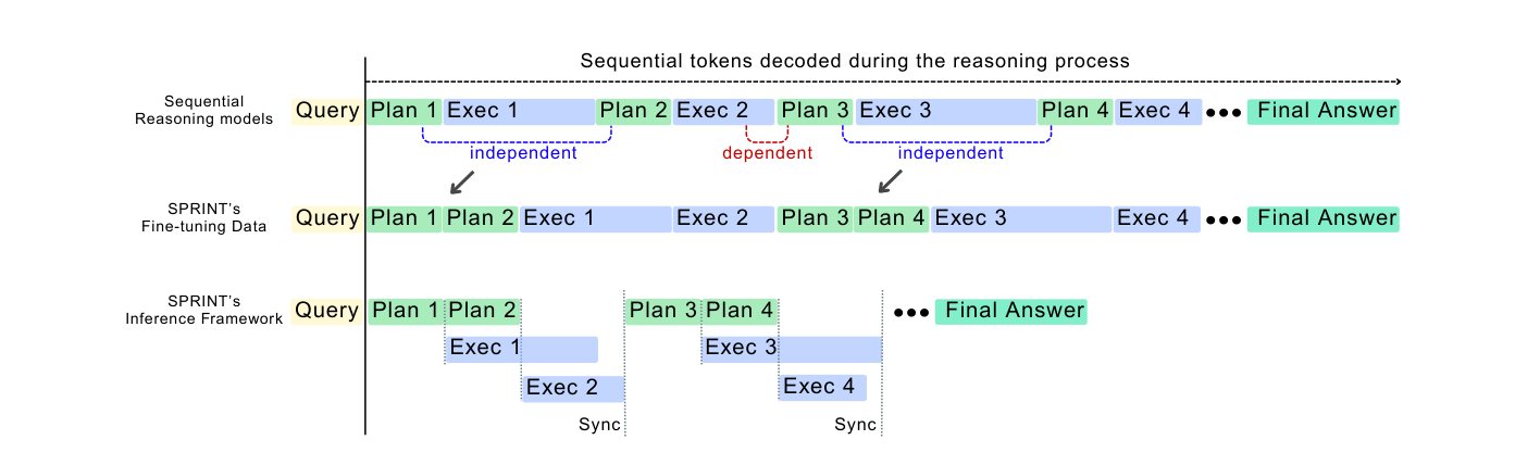
Figure 3 (SPRINT paper). Notice the bottom timeline: independent executions stack vertically (concurrent) instead of extending the line, and each stage ends at a Sync. Same steps, visibly shorter critical path.
| Dimension | Conventional serial LRM / trajectory RL | SPRINT |
|---|---|---|
| Training unit | whole trajectory | a stage (combined plan + concurrent executions) |
| Trajectory handling | one serial chain, unaltered | restructured into a partially parallel stage graph |
| Credit assignment | reward spread over the chain (RL) / imitate the chain (SFT) | none needed — pure imitation of the layout |
| Feedback | reward or golden target | supervised target sequence; sync ≠ reward |
| Data efficiency | one example per trajectory | one example per trajectory, but each teaches structure (same ~1,700 traces beat RFT) |
| Long-horizon learning | latency grows with chain length | critical path shrinks as independence grows |
| Engineering complexity | decoding loop | decoding loop + orchestrator + curation pipeline |
The measured payoff (paper’s numbers; sequential tokens, not total):
| Benchmark | Baseline (RFT) | SPRINT | Seq-token reduction |
|---|---|---|---|
| MATH-500 (in-domain) | 91.0% · 2,880 | 92.5% · 2,440 | ~15% |
| Countdown (OOD) | 84.9% · 4,917 | 85.9% · 2,284 | ~53% |
| GPQA-Diamond (OOD) | 50.5% · 7,103 | 51.0% · 6,336 | ~11% |
Three honest qualifiers, all from the paper. (1) SPRINT often generates more total tokens (e.g. MATH: 3,622 total vs. 2,440 sequential) — the win is critical-path length, not total work. (2) On the shortest problems the fixed protocol overhead makes SPRINT ~5% worse; the savings scale with trajectory length (up to ~39% on problems needing >8,000 tokens, and 45%/65% on the long-trajectory slices of GPQA/Countdown). (3) Wall-clock gains (~9% on MATH, ~38% on long chains) are smaller than the token reduction, because the optimal hardware-parallel serving system was not built. Do not claim superiority beyond that: SPRINT matches reasoning accuracy while cutting sequential tokens — it is a latency method, not an accuracy method (the small accuracy bumps come from error isolation across independent branches).
14. SPRINT vs. SWiRL
Both restructure multi-step reasoning for training, and they even share a co-author (Azalia Mirhoseini) — but they solve different problems and must not be conflated. See the full build in the SWiRL engineering implementation.
| SWiRL | SPRINT | |
|---|---|---|
| Problem it addresses | quality of each decision in a tool-using agent trajectory | latency of long serial reasoning (too many sequential tokens) |
| Trajectory type | environment-interaction: reason → tool call → observation → … | pure reasoning trace (no tools in-paper) |
| How it structures experience | decompose a trajectory into per-step state → action units |
restructure a trace into plan/execution stages via a dependency DAG |
| Training mechanism | step-wise RL — a reward $R(a\mid s)$ on every action, optimized by policy gradient | plain SFT — next-token loss on the reformatted sequence; no reward |
| Selection signal | process filtering (a judge scores each step’s reasonableness) | correctness filter on raw traces + parallelization-ratio ≥ 1.5 |
| Changes inference? | no — improves each step; loop stays sequential | yes — emits a parallel structure the orchestrator runs concurrently |
| What it optimizes | expected step-wise reward | reproducing a parallelizable layout |
The one-line distinction: SWiRL makes each step better; SPRINT makes independent steps concurrent. SWiRL keeps the loop sequential and sharpens per-step decision quality with reward; SPRINT keeps accuracy roughly fixed and shortens the critical path with a learned plan/parallel layout. They are, in principle, composable — you could sharpen steps and parallelize independent ones — but the paper does neither combine them nor claim to.
15. Where This Sits in the Post-Training Landscape
SPRINT is a post-training stage: it takes a model that already reasons (via prior reasoning fine-tuning) and teaches that reasoning a new shape. It is not a replacement for reasoning training, and — as §7 stressed — it is not an RL method. For the broader background on how reward-based post-training actually works — RLHF, RLAIF, RLVF, RLEF, SWiRL, and where PPO, GRPO, and DPO fit by feedback source — see the companion blog:
Reinforcement Learning for LLMs: RLHF, RLAIF, RLVF, RLEF & SWiRL Post-Training Explained
The raw material for SPRINT is DeepSeek-R1 reasoning traces; the DeepSeek-R1 engineering implementation covers how those reasoning trajectories are produced in the first place. This article explains how you would build SPRINT; those two cover the training substrate it consumes and the reward machinery it deliberately avoids.
Key Takeaways
- SPRINT is a data-transformation + orchestration method, not a new optimizer or kernel. It post-trains a reasoning model, via ordinary SFT, to emit an interleaved plan → parallel-execution → sync trajectory.
- The parallelism is at the reasoning level. A planner proposes independent subtasks; a pool of executors (the same model) runs them concurrently; results sync into a shared context. Turning that logical parallelism into wall-clock speedup is a separate, unsolved systems problem.
- Parallelism is read off a dependency DAG, never off textual order. Steps are extracted into plan/execution phases, wired into $G=(S,D)$, and packed into stages by the $\sigma(S_i)$ recurrence — with a plan-only-parent optimization that packs tighter.
- The optimized quantity is sequential tokens. SPRINT can generate more total tokens while cutting the critical path; savings scale with trajectory length (up to ~39% beyond 8k tokens; ~5% overhead on short problems).
- There is no reward. Correctness filtering only selects raw traces; the training signal is next-token loss on the restructured sequence. This is the sharpest line between SPRINT and reward-based methods like SWiRL, PPO, and GRPO.
- It preserves dependencies by design. SPRINT turns a partially sequential computation graph into a partially parallel execution graph — branching where reasoning is independent, staying serial where it isn’t.