Fig. 03 — Signal dossier / 2026.10
Accelerating Mamba-2 with High-Performance Forward Pass Kernels in NVIDIA CUDA Tile
Accelerate Mamba-2 with high-performance forward pass kernels in NVIDIA CUDA Tile: how the SSD chunked scan maps to GPU tiles for faster training and inference.
- Published
- 23 Oct 2026signal no. 03
- Category
- GPU Kernelsfield note
- Read time
- 22 min~4698 words
- Topics
- Mamba-2+ 3 more
- Author
- Trisham Patilindependent reading
Filed 2026-10-23 Signal no. 03GPU Kernels Read time: 22 min
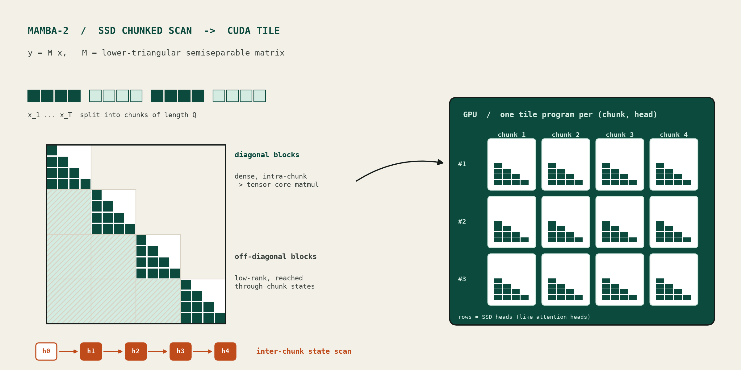 The Mamba-2 SSD chunked scan as GPU tiles: dense intra-chunk blocks run as tensor-core matmuls, and a short state scan carries information between chunks. Drawn for this post.
NVIDIA CUDA Tile (cuTile) is a Python DSL for writing GPU kernels at the level of tiles (blocks of data) instead of individual threads and warps. You describe what happens to each tile, and the compiler handles the scheduling and maps the heavy math onto hardware like Tensor Cores. You write the kernel in Python, and the compiler gets it to near hand-tuned speed.
Jane Street, the quantitative trading firm, was one of cuTile’s early adopters. Its machine learning engineers implemented Mamba-2, a state-of-the-art sequence model, in cuTile, and then worked with NVIDIA to optimize the kernels. This post walks through the three custom kernels behind the Mamba-2 forward pass and the cuTile optimizations that make them fast.
Why Would a Trading Firm Care About Mamba-2 Kernels?
Jane Street uses deep learning for quantitative research. It hasn’t said which models run in production, but it’s easy to see why Mamba-2 fits that work:
- Markets are long sequences. Order books, trades and prices arrive as streams of events, and the signal is often spread across thousands of steps of history. Attention’s cost grows quadratically with sequence length; Mamba-2 grows linearly, so longer look-back windows stay affordable.
- Streaming inference is cheap. At inference time, Mamba-2 carries a fixed-size state forward and updates it with each new event, instead of re-reading the whole history. That’s a natural shape for models that react to live market data.
- Faster kernels mean more experiments. Quant research is a loop of training, testing and discarding ideas. A faster forward pass means more model variants tested on the same GPUs in the same time.
- Python stays the research language. With cuTile, the people designing the models can also write and tune the kernels, without handing them off to a separate CUDA C++ team.
From Classical Statistics to Deep Learning: How Time Series Forecasting Evolved
When tackling time series forecasting and sequential data, our approach has evolved significantly over the years. Here is how we moved from traditional statistical models to deep learning architectures with built-in memory, the line of work that leads to state space models like Mamba-2.
1. The Classical Foundations: Random Walk, AR, ARIMA and SARIMAX
For standard time series forecasting, we typically lean on classical statistical models.
Random Walk. The simplest baseline: tomorrow’s value is today’s value plus noise. It’s the benchmark every forecasting model has to beat.
\[y_t = y_{t-1} + \varepsilon_t, \qquad \varepsilon_t \sim \mathcal{N}(0, \sigma^2)\]AR (Autoregressive) models. Great for baseline forecasting and capturing basic linear trends. An AR($p$) model predicts the next value as a weighted sum of the last $p$ values:
\[y_t = c + \sum_{i=1}^{p} \phi_i \, y_{t-i} + \varepsilon_t\]ARIMA and SARIMAX. These account for differencing (the “I”, which removes trends), moving averages of past errors (the “MA”) and, in SARIMAX, seasonality and exogenous variables (the “S” and the “X”). Using the lag operator $L$, where $L y_t = y_{t-1}$, an ARIMA($p, d, q$) model is:
\[\Big(1 - \sum_{i=1}^{p} \phi_i L^i\Big)(1 - L)^d \, y_t = c + \Big(1 + \sum_{j=1}^{q} \theta_j L^j\Big)\varepsilon_t\]SARIMAX($p, d, q$)($P, D, Q$)$_s$ adds seasonal polynomials at period $s$ (for example, $s = 7$ for daily data with a weekly cycle) and a regression term on external inputs $x_t$:
\[\Phi_P(L^s)\,\phi_p(L)\,(1 - L)^d (1 - L^s)^D \, y_t = \beta^\top x_t + \Theta_Q(L^s)\,\theta_q(L)\,\varepsilon_t\]The limitation. These models work well for many short- to medium-term tasks, but they struggle when important patterns are buried deep in the past. Every model above looks back a fixed number of lags ($p$, $q$, $P$, $Q$) and assumes the relationships are linear, so very long-range dependencies are hard to capture.
2. Enter Recurrent Neural Networks (RNNs)
To handle large amounts of sequential data and learn complex patterns across time steps, Recurrent Neural Networks (RNNs) enter the picture. Unlike static models, an RNN keeps a hidden state $h_t$ that carries information from one step to the next, so it can read chronological data in order:
\[h_t = \tanh\big(W_h h_{t-1} + W_x x_t + b\big), \qquad \hat{y}_t = W_y h_t + b_y\]The same weights are reused at every step, and the hidden state is the model’s only memory of the past.
3. Solving Long-Term Memory with LSTMs and GRUs
Standard RNNs struggle with vanishing gradients. During training, the gradient that links step $T$ back to an earlier step $k$ is a long product of Jacobians:
\[\frac{\partial h_T}{\partial h_k} = \prod_{t=k+1}^{T} \frac{\partial h_t}{\partial h_{t-1}}\]If those factors are mostly smaller than 1, the product shrinks towards zero, and the network can’t learn from information many steps back. This is where LSTMs (Long Short-Term Memory networks) and GRUs (Gated Recurrent Units) shine.
The power of gates. Gating mechanisms (forget, input and output gates) let the model decide what to keep and what to discard. Each gate is a sigmoid $\sigma$ that outputs values between 0 (block) and 1 (pass), and $\odot$ is element-wise multiplication. The LSTM:
\[\begin{aligned} f_t &= \sigma(W_f x_t + U_f h_{t-1} + b_f) && \text{forget gate} \\ i_t &= \sigma(W_i x_t + U_i h_{t-1} + b_i) && \text{input gate} \\ o_t &= \sigma(W_o x_t + U_o h_{t-1} + b_o) && \text{output gate} \\ \tilde{c}_t &= \tanh(W_c x_t + U_c h_{t-1} + b_c) && \text{candidate memory} \\ c_t &= f_t \odot c_{t-1} + i_t \odot \tilde{c}_t && \text{cell state} \\ h_t &= o_t \odot \tanh(c_t) && \text{hidden state} \end{aligned}\]The GRU does the same job with two gates, an update gate $z_t$ and a reset gate $r_t$, and no separate cell state:
\[\begin{aligned} z_t &= \sigma(W_z x_t + U_z h_{t-1} + b_z) \\ r_t &= \sigma(W_r x_t + U_r h_{t-1} + b_r) \\ \tilde{h}_t &= \tanh\big(W_h x_t + U_h (r_t \odot h_{t-1}) + b_h\big) \\ h_t &= (1 - z_t) \odot h_{t-1} + z_t \odot \tilde{h}_t \end{aligned}\]Built-in memory. The key line is the LSTM cell update $c_t = f_t \odot c_{t-1} + i_t \odot \tilde{c}_t$. It’s additive: when the forget gate stays near 1, the old memory passes through almost unchanged, and gradients flow back through it without vanishing. These models act as systems with dynamic, built-in memory, so relevant context from long ago still shapes future predictions.
Summary: From Linear Models to Learned Memory
Classical linear models set the stage for forecasting. Deep learning architectures like LSTMs and GRUs bridge the gap with non-linear learning and learned memory management for complex sequential data.
There’s still one catch. LSTMs and GRUs process a sequence one step at a time, because each $h_t$ depends on $h_{t-1}$. That makes them slow to train on GPUs, which are built for parallel work. Fixing that without giving up the memory is the problem state space models like Mamba-2 set out to solve. For the first-generation design, see the Mamba selective state spaces breakdown.
Mamba-2 and State Space Duality: Recurrent Memory at Matmul Speed
The Sequence Modeling Trade-Off: Attention vs RNNs
Every sequence architecture has to pick a side in a compute trade-off:
| Softmax attention | RNNs | Mamba-2 | |
|---|---|---|---|
| Training | Fast: big matmuls on Tensor Cores | Slow: one step at a time, can’t parallelize | Fast: chunked matmuls on Tensor Cores |
| Inference cost per token | Grows with sequence length (the KV cache keeps growing) | Constant | Constant |
| Memory at inference | Grows linearly with context | Fixed | Fixed-size state |
Mamba-2 belongs to a family of models that aim for the best of both. Like an RNN, it has a fixed-size hidden state and a recurrent update. Unlike an RNN, that update can be computed chunk by chunk with Tensor Core matmuls.
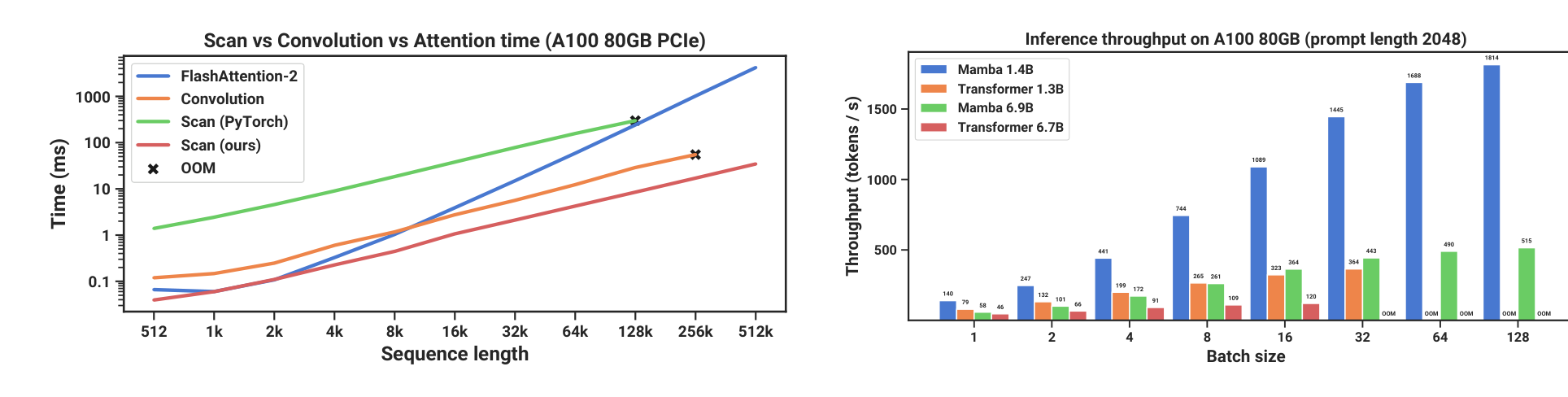 Figure 8 from the Mamba paper: the original Mamba-1 selective scan against attention. Mamba-2’s SSD algorithm goes further by turning most of that scan into matmuls. Read more here →
The Mamba-2 Recurrence
The core recurrence of a Mamba-2 head is:
\[h_t = \exp(A \cdot dt_t)\, h_{t-1} + dt_t\, B_t\, x_t^\top, \qquad y_t = c_t^\top h_t + D\, x_t\]Where:
- $x_t$, $dt_t$, $B_t$ and $c_t$ are the layer’s inputs at token $t$. Like queries, keys and values in attention, they come from projecting the block’s input.
- $y_t$ is the output at token $t$.
- $h_t$ is the fixed-size hidden state carried from token to token. Unlike an RNN’s state, it’s a matrix, not a vector, so it holds more numbers and has more representational capacity.
- $A$ and $D$ are learned parameters.
The intuition for each input:
- $dt_t$ (one scalar per head) controls how much the state updates at this token. It’s always positive, and $A$ is always negative, so the decay factor $\exp(A \cdot dt_t)$ lies between 0 and 1. When $dt_t = 0$, the decay is $\exp(0) = 1$ and nothing new is written, so the state passes through unchanged.
- $x_t$ (a vector of size $H$) plays the role of the values in attention.
- $B_t$ (a vector of size $S$) plays the role of the keys.
- $c_t$ (a vector of size $S$) decides how the state is read out, the role of the queries.
The state $h_t$ has shape $(S, H)$, because $B_t x_t^\top$ is an outer product. To keep the algebra short, write $a_t = A \cdot dt_t$ (always negative) and $b_t = dt_t B_t$:
\[h_t = \exp(a_t)\, h_{t-1} + b_t x_t^\top, \qquad y_t = c_t^\top h_t + D\, x_t\]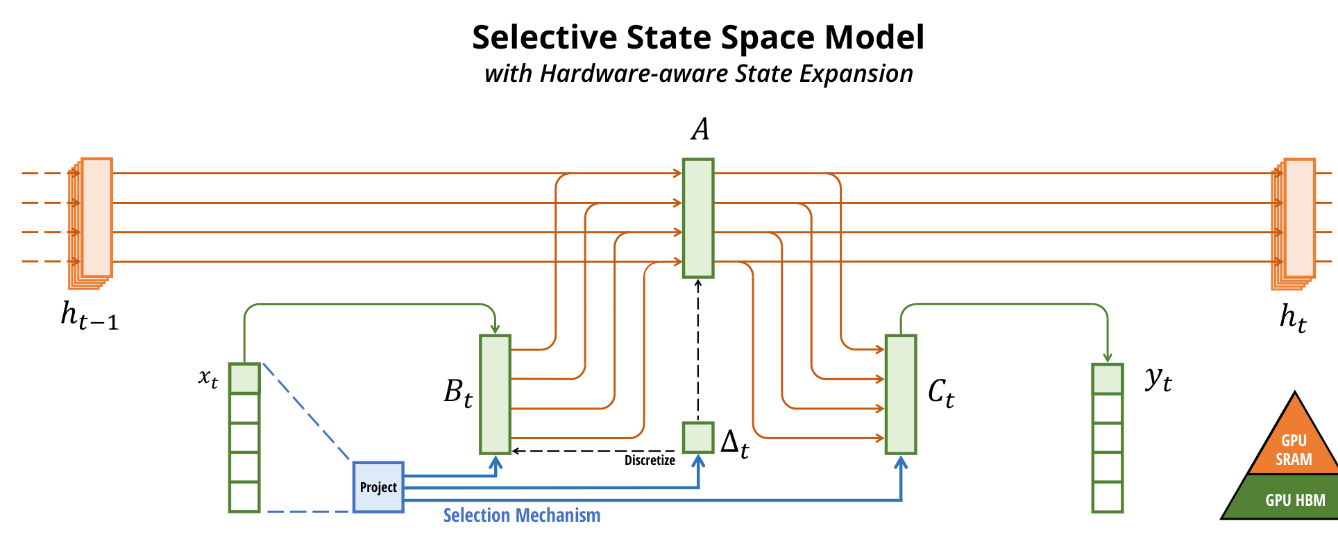 Figure 1 from the Mamba paper: each channel maps through a much larger hidden state. Keeping that state out of slow GPU memory is the whole engineering problem. Read more here →
Why a Parallel Scan Isn’t Enough
The recurrence is perfect for generating one token at a time. Training and prefill, though, process thousands of tokens at once and need something faster than a for-loop.
Because the state update is linear, it can run as a parallel scan. But a scan has to materialize a huge hidden-state tensor, one $(S, H)$ matrix per token. That makes it memory-bound, and it can’t use Tensor Cores at all. Read more here →
Step 1: Jump the State Across a Chunk with One Matmul
The alternative is to compute a future state directly with a matrix multiply. Ignore the decay $\exp(a_t)$ for a moment. Going from $h_t$ to $h_{t+T}$ just adds up $T$ outer products:
\[h_{t+T} = h_t + b_{t+1} x_{t+1}^\top + b_{t+2} x_{t+2}^\top + \cdots + b_{t+T} x_{t+T}^\top\]Stack the $b_{t+i}$ as rows of a matrix $B$ with shape $(T, S)$, and the $x_{t+i}$ as rows of $X$ with shape $(T, H)$. The whole sum becomes one matmul:
\[h_{t+T} = h_t + B^\top X\]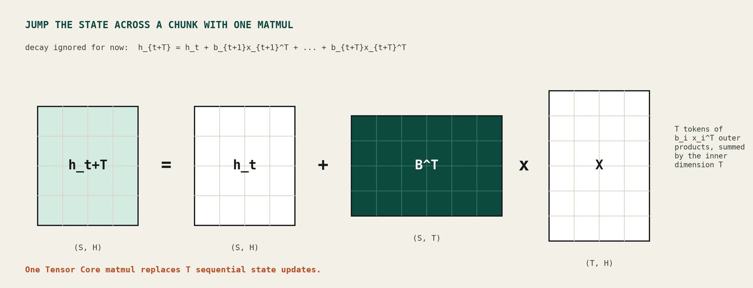 Jumping the hidden state across a chunk of $T$ tokens with one matmul (decay ignored). Drawn for this post.
With this jump formula, you can cheaply compute the hidden state at chunk checkpoints along the sequence.
Step 2: Compute a Chunk of Outputs from One State
Next, compute the outputs $y_{t+1}, \dots, y_{t+T}$ given only the chunk’s starting state $h_t$. Computing every intermediate state would defeat the point of the jump. So expand each state instead (still without decay):
\[y_{t+i} = c_{t+i}^\top h_{t+i} + D x_{t+i} = c_{t+i}^\top \big(h_t + b_{t+1} x_{t+1}^\top + \cdots + b_{t+i} x_{t+i}^\top\big) + D x_{t+i}\]Output $y_{t+i}$ only sees the $b_j$ for $j \le t + i$. Stack the chunk’s $c$, $b$, $x$ and $y$ into matrices $C$, $B$, $X$ and $Y$, and those past-only terms become a causal mask $M$ on the product $CB^\top$:
\[Y = C\, h_t + \big((C B^\top) \odot M\big) X + D X\]This looks like attention without the softmax, and that’s no accident. Without the decay term, Mamba-2 is linear attention under different names. For that connection, read more here →
Step 3: Add Back the Decay, Safely, in Log-Space
With decay, each term picks up the product of every decay factor after it:
\[h_{t+T} = e^{a_{t+1} + \cdots + a_{t+T}}\, h_t + e^{a_{t+2} + \cdots + a_{t+T}}\, b_{t+1} x_{t+1}^\top + \cdots + b_{t+T} x_{t+T}^\top\]Working in log-space turns those products into cumulative sums. Let $g$ hold the cumulative sum of $a$ inside the chunk, and let $g_{\text{last}}$ be its final value. Scaling the rows of $B$ by their exponentials keeps the jump a single matmul:
\[h_{t+T} = e^{g_{\text{last}}}\, h_t + \big(e^{g_{\text{last}} - g} \odot B\big)^\top X\]Plugging that into the output equation gives the full chunk computation:
\[Y = \big(e^{g} \odot C h_t\big) + \big(L \odot C B^\top\big) X + D X, \qquad L_{ij} = \begin{cases} e^{g_i - g_j} & i \ge j \\ 0 & i < j \end{cases}\]This is also numerically safe. Every $a_t$ is negative, so for every kept entry ($i \ge j$), $g_i - g_j = a_{j+1} + \cdots + a_i \le 0$. The exponent can only shrink values towards zero. The entries where it would be positive, and could overflow, are exactly the future entries the causal mask throws away.
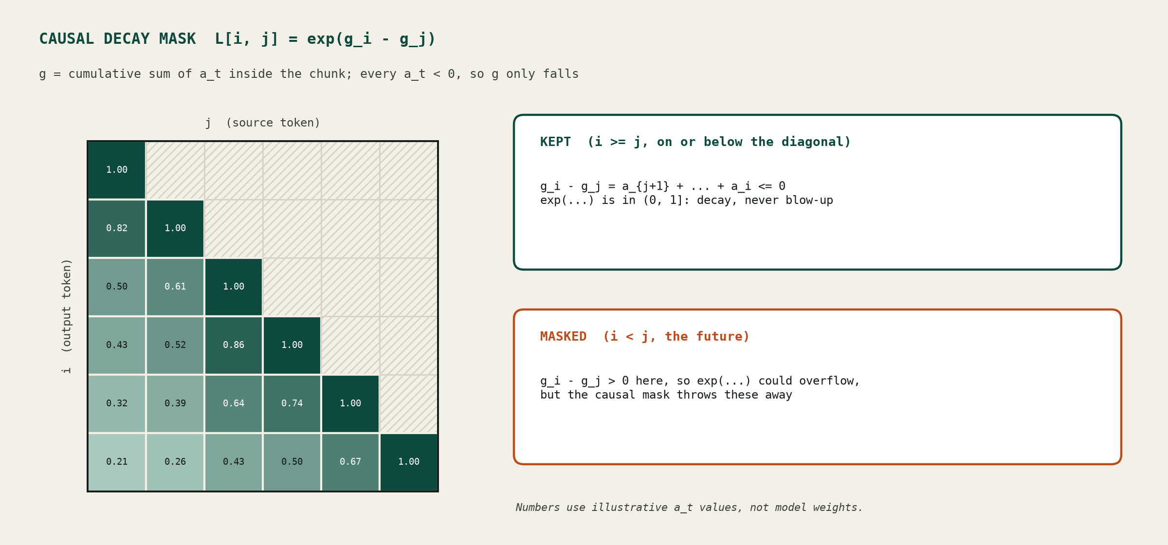 The decay mask $L$ for a 6-token chunk with illustrative values. Every kept entry is at most 1, and the masked entries are the only ones that could blow up. Drawn for this post.
From the Math to Three Kernels
This derivation maps onto three GPU kernels:
Kernel 01 / Prep
chunk_cumsum
Computes the cumulative sums of at inside each chunk: the g used by both later kernels.
Kernel 02 / State
fwd_pass_state
Walks the chunks in order, applying the jump formula to get the hidden state at the start of each chunk.
Kernel 03 / Output
compute_out
Computes every chunk's outputs in parallel from its starting state, with the decay mask fused in.
The Three Mamba-2 Forward Pass Kernels in cuTile (with Triton Side by Side)
Each kernel below shows the cuTile code on the left and a Triton version of the same kernel on the right.
About the code. The cuTile kernels come from NVIDIA and Jane Street’s implementation in TileGym. Their write-up shows kernels 2 and 3 as fragments, so the signatures here are reconstructed from the variables the bodies use. The Triton versions are sketches written for this post to mirror each cuTile kernel line for line. They aren’t the
mamba_ssmreference kernels, which split the same work across more kernels (chunk cumsum, chunk state, state passing, the $CB^\top$ product and chunk scan).
The biggest difference is visible straight away. cuTile addresses tiles by index: ct.load(x, index=..., shape=...) fetches a whole tile, with padding handled for you. Triton works with pointers: you build every tile’s address from offsets and strides, and you write the bounds masks by hand.
Kernel 1: chunk_cumsum, the Cumulative Decay Sums
Kernels 2 and 3 both need $g$, the cumulative sum of $a_t = A \cdot dt_t$. So this kernel computes it once and stores it. It’s a cumulative sum within each chunk, not across the whole sequence.
Its inputs are a per-head scalar decay a and a per-token, per-head timestep dt. The effective decay for head $h$ at token $t$ is a[h] * dt[t, h], and the kernel accumulates it along the chunk. Every later use takes an exponential of these sums, and exp2 is cheaper than exp, so the result is pre-scaled by $\log_2 e$. That works because $e^{x} = 2^{x \log_2 e}$.
This kernel introduces the cuTile primitives all three kernels share: ct.bid (where am I in the grid?), ct.load / ct.store (move a whole tile) and ct.cumsum.
cuTile
@ct.kernel
def chunk_cumsum_kernel(
    a: torch.Tensor,       # [num_heads]
    dt: torch.Tensor,      # [batch, num_tokens, num_heads]
    output: torch.Tensor,  # [batch, num_tokens, num_heads]
    chunk_size: ct.Constant[int],
    BLOCK_H: ct.Constant[int],
) -> None:
    chunk_idx, head_tile_idx, batch = ct.bid(0), ct.bid(1), ct.bid(2)
    dt_tile = ct.load(dt, index=(batch, chunk_idx, head_tile_idx),
                      shape=(1, chunk_size, BLOCK_H),
                      padding_mode=ct.PaddingMode.ZERO).astype(ct.float32)
    a_tile = ct.load(a, index=(head_tile_idx,),
                     shape=(BLOCK_H,),
                     padding_mode=ct.PaddingMode.ZERO).astype(ct.float32)

    d_tile = ct.cumsum(a_tile * dt_tile, axis=1) * LOG2E
    ct.store(output, index=(batch, chunk_idx, head_tile_idx),
             tile=d_tile.astype(output.dtype))
Triton (sketch)
LOG2E: tl.constexpr = 1.4426950408889634

@triton.jit
def chunk_cumsum_kernel(
    a_ptr, dt_ptr, out_ptr, num_tokens, num_heads,
    s_b, s_t, s_h,  # dt / output strides
    CHUNK_SIZE: tl.constexpr, BLOCK_H: tl.constexpr,
):
    chunk, head_tile, batch = (tl.program_id(0), tl.program_id(1),
                               tl.program_id(2))
    offs_t = chunk * CHUNK_SIZE + tl.arange(0, CHUNK_SIZE)
    offs_h = head_tile * BLOCK_H + tl.arange(0, BLOCK_H)
    mask = (offs_t[:, None] < num_tokens) & (offs_h[None, :] < num_heads)
    ptrs = batch * s_b + offs_t[:, None] * s_t + offs_h[None, :] * s_h

    dt = tl.load(dt_ptr + ptrs, mask=mask, other=0.0).to(tl.float32)
    a = tl.load(a_ptr + offs_h, mask=offs_h < num_heads,
                other=0.0).to(tl.float32)

    d = tl.cumsum(a[None, :] * dt, axis=0) * LOG2E
    tl.store(out_ptr + ptrs, d, mask=mask)
The kernel launches on a grid of (num_chunks, num_head_tiles, batch_size), and ct.bid gives each program its coordinates. Broadcasting a_tile (shape [BLOCK_H]) against dt_tile (shape [1, chunk_size, BLOCK_H]) gives the per-token, per-head decay across the tile. Then ct.cumsum(..., axis=1) scans along the tokens of the chunk, and the result is stored in the layout the next two kernels expect.
Kernel 2: fwd_pass_state, Carrying the State Between Chunks
fwd_pass_state computes the starting hidden state of every chunk, plus the final state after the last chunk. It doesn’t produce outputs. It prepares the carried state that compute_out will later turn into outputs.
At its core, it’s the sequential loop over chunks from the jump formula. Each program owns one (batch, head, head_tile, state_tile) slice of the state, held as hid_tile with shape [BLOCK_HEAD, BLOCK_STATE]. In every iteration it:
- Stores the current state as this chunk’s starting state.
- Loads one chunk of
x,b,dtanddecay_cumsum. - Applies the jump, $h \leftarrow e^{g_{\text{last}}} h + \big(e^{g_{\text{last}} - g} \odot B\big)^\top X$.
ct.extract pulls the chunk’s last decay value ($g_{\text{last}}$) out of the tile, ct.exp2 replaces exp, and ct.mma runs the matrix multiply-accumulate on the Tensor Cores.
cuTile
@ct.kernel  # signature reconstructed from the body
def fwd_pass_state_kernel(x, b, dt, decay_cumsum, init_state,
                          hiddens, final_state,
                          chunk_size: ct.Constant[int],
                          num_heads_per_group: ct.Constant[int],
                          BLOCK_HEAD: ct.Constant[int],
                          BLOCK_STATE: ct.Constant[int]):
    head_tile_idx, state_tile_idx, batch_head = (
        ct.bid(0), ct.bid(1), ct.bid(2))
    batch = batch_head // x.shape[2]
    head = batch_head % x.shape[2]
    group = head // num_heads_per_group

    hid_tile = ct.load(
        init_state,
        index=(batch, head, head_tile_idx, state_tile_idx),
        shape=(1, 1, BLOCK_HEAD, BLOCK_STATE),
    ).reshape((BLOCK_HEAD, BLOCK_STATE))

    num_chunks = ct.cdiv(b.shape[1], chunk_size)
    for chunk_idx in range(num_chunks):
        ct.store(
            hiddens,
            index=(batch, head, chunk_idx, head_tile_idx, state_tile_idx),
            tile=hid_tile.reshape((1, 1, 1, BLOCK_HEAD, BLOCK_STATE))
                         .astype(hiddens.dtype),
        )
        x_tile = ct.load(
            x, index=(batch, chunk_idx, head, head_tile_idx),
            shape=(1, chunk_size, 1, BLOCK_HEAD),
            padding_mode=ct.PaddingMode.ZERO,
        ).reshape((chunk_size, BLOCK_HEAD))
        b_tile = ct.load(
            b, index=(batch, chunk_idx, group, state_tile_idx),
            shape=(1, chunk_size, 1, BLOCK_STATE),
            padding_mode=ct.PaddingMode.ZERO,
        ).reshape((chunk_size, BLOCK_STATE))
        dt_tile = ct.load(
            dt, index=(batch, chunk_idx, head),
            shape=(1, chunk_size, 1),
            padding_mode=ct.PaddingMode.ZERO,
        ).reshape((chunk_size,))
        d_tile = ct.load(
            decay_cumsum, index=(batch, chunk_idx, head),
            shape=(1, chunk_size, 1),
            padding_mode=ct.PaddingMode.ZERO,
        ).reshape((chunk_size,))
        d_last = ct.extract(d_tile, index=(chunk_size - 1,),
                            shape=(1,))

        b_dt_d = b_tile * (dt_tile * ct.exp2(d_last - d_tile))[:, None]
        hid_tile = ct.exp2(d_last) * hid_tile
        hid_tile = ct.mma(x_tile.transpose(),
                          b_dt_d.astype(b.dtype), hid_tile)

    ct.store(
        final_state,
        index=(batch, head, head_tile_idx, state_tile_idx),
        tile=hid_tile.reshape((1, 1, BLOCK_HEAD, BLOCK_STATE)),
    )
Triton (sketch)
@triton.jit
def fwd_pass_state_kernel(
    x_ptr, b_ptr, dt_ptr, dcs_ptr, init_ptr, hid_ptr, final_ptr,
    num_tokens, num_heads, heads_per_group,
    sx_b, sx_t, sx_h, sx_p,          # x:  [batch, token, head, P]
    sb_b, sb_t, sb_g, sb_s,          # b:  [batch, token, group, S]
    sd_b, sd_t, sd_h,                # dt, decay_cumsum
    sh_b, sh_h, sh_c, sh_p, sh_s,    # hiddens
    si_b, si_h, si_p, si_s,          # init_state, final_state
    CHUNK_SIZE: tl.constexpr,
    BLOCK_HEAD: tl.constexpr, BLOCK_STATE: tl.constexpr,
):
    head_tile, state_tile, batch_head = (
        tl.program_id(0), tl.program_id(1), tl.program_id(2))
    batch = batch_head // num_heads
    head = batch_head % num_heads
    group = head // heads_per_group

    offs_p = head_tile * BLOCK_HEAD + tl.arange(0, BLOCK_HEAD)
    offs_s = state_tile * BLOCK_STATE + tl.arange(0, BLOCK_STATE)
    offs_c = tl.arange(0, CHUNK_SIZE)
    state_off = (batch * si_b + head * si_h
                 + offs_p[:, None] * si_p + offs_s[None, :] * si_s)
    hid = tl.load(init_ptr + state_off).to(tl.float32)

    for chunk in range(tl.cdiv(num_tokens, CHUNK_SIZE)):
        tl.store(hid_ptr + batch * sh_b + head * sh_h + chunk * sh_c
                 + offs_p[:, None] * sh_p + offs_s[None, :] * sh_s,
                 hid.to(hid_ptr.dtype.element_ty))

        offs_t = chunk * CHUNK_SIZE + offs_c
        t_ok = offs_t < num_tokens
        x = tl.load(x_ptr + batch * sx_b + offs_t[:, None] * sx_t
                    + head * sx_h + offs_p[None, :] * sx_p,
                    mask=t_ok[:, None], other=0.0)
        b = tl.load(b_ptr + batch * sb_b + offs_t[:, None] * sb_t
                    + group * sb_g + offs_s[None, :] * sb_s,
                    mask=t_ok[:, None], other=0.0)
        tok = batch * sd_b + offs_t * sd_t + head * sd_h
        dt = tl.load(dt_ptr + tok, mask=t_ok, other=0.0)
        d = tl.load(dcs_ptr + tok, mask=t_ok, other=0.0)
        d_last = tl.sum(tl.where(offs_c == CHUNK_SIZE - 1, d, 0.0))

        b_dt_d = b * (dt * tl.exp2(d_last - d))[:, None]
        hid = hid * tl.exp2(d_last)
        hid = tl.dot(tl.trans(x), b_dt_d.to(x.dtype), hid)

    tl.store(final_ptr + state_off, hid)
After the last chunk, hid_tile holds the final hidden state, which gets stored. At inference you can feed it back in as the next call’s init_state. During training it’s usually discarded.
The key design point: the sequential dependence stays inside one program instance. Each program walks its chunks in order, while the independent (batch, head, head_tile, state_tile) slices run in parallel across the grid.
Kernel 3: compute_out, the Fused Output Kernel
compute_out is the last kernel in the forward pass. It takes each chunk’s starting state from fwd_pass_state and produces the token outputs with the output equation:
A direct PyTorch version would compute the three terms separately and write the full [batch, n_chunks, chunk_size, chunk_size] interaction matrix C @ B.T to global memory. compute_out fuses everything into one tiled kernel, and that matrix never leaves registers.
Each program owns one (batch, chunk, head, head_tile) output tile and works in two phases:
- Phase 1 loops over state tiles. It uses
ct.mmato build the interaction matrixcb_tile = C @ B.Tand, in the same loop, accumulates the carried-state termC @ H.T. - Phase 2 applies the pairwise decay and the causal mask to
cb_tile, then adds every term into the output tile.ct.arangeandct.wherebuild the lower-triangular mask on the fly, so no mask tensor is ever stored. The finalct.mmacasts toct.tfloat32to run on Tensor Cores at close to FP32 accuracy.
cuTile
@ct.kernel  # signature reconstructed from the body
def compute_out_kernel(x, b, c, dt, decay_cumsum, hiddens, d, out,
                       chunk_size: ct.Constant[int],
                       state_size: ct.Constant[int],
                       num_heads_per_group: ct.Constant[int],
                       BLOCK_HEAD: ct.Constant[int],
                       BLOCK_STATE: ct.Constant[int]):
    chunk_idx, head_tile_idx, batch_head = (
        ct.bid(0), ct.bid(1), ct.bid(2))
    batch = batch_head // x.shape[2]
    head = batch_head % x.shape[2]
    group = head // num_heads_per_group

    cb_tile = ct.full((chunk_size, chunk_size), 0.0, dtype=ct.float32)
    out_tile = ct.full((chunk_size, BLOCK_HEAD), 0.0, dtype=ct.float32)

    # Phase 1: build CB = C @ B.T, accumulate the carried-state output
    for state_tile_idx in range(state_size // BLOCK_STATE):
        b_tile = ct.load(
            b, index=(batch, chunk_idx, group, state_tile_idx),
            shape=(1, chunk_size, 1, BLOCK_STATE),
            padding_mode=ct.PaddingMode.ZERO,
        ).reshape((chunk_size, BLOCK_STATE))
        c_tile = ct.load(
            c, index=(batch, chunk_idx, group, state_tile_idx),
            shape=(1, chunk_size, 1, BLOCK_STATE),
            padding_mode=ct.PaddingMode.ZERO,
        ).reshape((chunk_size, BLOCK_STATE))
        h_tile = ct.load(
            hiddens,
            index=(batch, head, chunk_idx, head_tile_idx, state_tile_idx),
            shape=(1, 1, 1, BLOCK_HEAD, BLOCK_STATE),
        ).reshape((BLOCK_HEAD, BLOCK_STATE))

        cb_tile = ct.mma(c_tile, b_tile.transpose(), cb_tile)
        out_tile = ct.mma(c_tile,
                          h_tile.transpose().astype(c_tile.dtype),
                          out_tile)

    # Phase 2: decay + causal mask, then the final computation
    d_tile = ct.load(decay_cumsum, index=(batch, chunk_idx, head),
                     shape=(1, chunk_size, 1),
                     padding_mode=ct.PaddingMode.ZERO
                     ).reshape((chunk_size,))
    dt_tile = ct.load(dt, index=(batch, chunk_idx, head),
                      shape=(1, chunk_size, 1),
                      padding_mode=ct.PaddingMode.ZERO
                      ).reshape((chunk_size,))
    x_tile = ct.load(x, index=(batch, chunk_idx, head, head_tile_idx),
                     shape=(1, chunk_size, 1, BLOCK_HEAD),
                     padding_mode=ct.PaddingMode.ZERO
                     ).reshape((chunk_size, BLOCK_HEAD))
    d_val = ct.load(d, index=(head,), shape=(1,))

    cb_tile = cb_tile * ct.exp2(d_tile[:, None] - d_tile[None, :])
    idx = ct.arange(chunk_size, dtype=ct.int32)
    cb_tile = ct.where(idx[:, None] >= idx[None, :], cb_tile, 0.0)
    out_tile = out_tile * ct.exp2(d_tile[:, None])

    dt_x = dt_tile[:, None] * x_tile
    out_tile = ct.mma(cb_tile.astype(ct.tfloat32),
                      dt_x.astype(ct.tfloat32), out_tile)
    out_tile = out_tile + d_val * x_tile  # D * x skip
    ct.store(out, index=(batch, chunk_idx, head, head_tile_idx),
             tile=out_tile.reshape((1, chunk_size, 1, BLOCK_HEAD))
                          .astype(out.dtype))
Triton (sketch)
@triton.jit
def compute_out_kernel(
    x_ptr, b_ptr, c_ptr, dt_ptr, dcs_ptr, hid_ptr, d_ptr, out_ptr,
    num_tokens, num_heads, heads_per_group,
    sx_b, sx_t, sx_h, sx_p,          # x and out
    sb_b, sb_t, sb_g, sb_s,          # b and c
    sd_b, sd_t, sd_h,                # dt, decay_cumsum
    sh_b, sh_h, sh_c, sh_p, sh_s,    # hiddens
    CHUNK_SIZE: tl.constexpr, STATE_SIZE: tl.constexpr,
    BLOCK_HEAD: tl.constexpr, BLOCK_STATE: tl.constexpr,
):
    chunk, head_tile, batch_head = (
        tl.program_id(0), tl.program_id(1), tl.program_id(2))
    batch = batch_head // num_heads
    head = batch_head % num_heads
    group = head // heads_per_group

    offs_c = tl.arange(0, CHUNK_SIZE)
    offs_t = chunk * CHUNK_SIZE + offs_c
    t_ok = offs_t < num_tokens
    offs_p = head_tile * BLOCK_HEAD + tl.arange(0, BLOCK_HEAD)

    cb = tl.zeros((CHUNK_SIZE, CHUNK_SIZE), dtype=tl.float32)
    out = tl.zeros((CHUNK_SIZE, BLOCK_HEAD), dtype=tl.float32)

    # Phase 1: build CB = C @ B.T, accumulate the carried-state output
    for s0 in range(0, STATE_SIZE, BLOCK_STATE):
        offs_s = s0 + tl.arange(0, BLOCK_STATE)
        bc_off = (batch * sb_b + offs_t[:, None] * sb_t
                  + group * sb_g + offs_s[None, :] * sb_s)
        b = tl.load(b_ptr + bc_off, mask=t_ok[:, None], other=0.0)
        c = tl.load(c_ptr + bc_off, mask=t_ok[:, None], other=0.0)
        h = tl.load(hid_ptr + batch * sh_b + head * sh_h
                    + chunk * sh_c + offs_p[:, None] * sh_p
                    + offs_s[None, :] * sh_s)

        cb = tl.dot(c, tl.trans(b), cb)
        out = tl.dot(c, tl.trans(h).to(c.dtype), out)

    # Phase 2: decay + causal mask, then the final computation
    tok = batch * sd_b + offs_t * sd_t + head * sd_h
    dcs = tl.load(dcs_ptr + tok, mask=t_ok, other=0.0)
    dt = tl.load(dt_ptr + tok, mask=t_ok, other=0.0)
    x_off = (batch * sx_b + offs_t[:, None] * sx_t
             + head * sx_h + offs_p[None, :] * sx_p)
    x = tl.load(x_ptr + x_off, mask=t_ok[:, None], other=0.0)
    d_val = tl.load(d_ptr + head)

    cb = cb * tl.exp2(dcs[:, None] - dcs[None, :])
    cb = tl.where(offs_c[:, None] >= offs_c[None, :], cb, 0.0)
    out = out * tl.exp2(dcs[:, None])

    dt_x = (dt[:, None] * x).to(tl.float32)
    out = tl.dot(cb, dt_x, out, input_precision="tf32")
    out = out + d_val * x
    tl.store(out_ptr + x_off, out.to(out_ptr.dtype.element_ty),
             mask=t_ok[:, None])
One line deserves a second look: ct.exp2(d_tile[:, None] - d_tile[None, :]). It does compute some unsafe exponentials: the above-diagonal entries, where the exponent is positive. The very next line masks them to zero, so a potential overflow never makes it into the output. That’s the log-space safety argument from section 02, written in two lines of code.
Mamba-2 Performance Optimizations in cuTile
With the kernels written in cuTile, four optimizations take them from correct to fast:
Opt 01 / Scheduling
Latency hints
You can annotate ct.load and ct.store with latency hints that model DRAM traffic. The compiler uses them to plan instruction scheduling and how deep to make the pipeline buffers.
Opt 02 / Tensor Cores
Swap A/B
On Blackwell's fifth-generation Tensor Cores, the two MMA operands aren't equal: A can live in Tensor Memory, but B must sit in shared memory. In fwd_pass_state, the identity BTAT = (AB)T routes the fused, freshly computed operand (b_dt_d) to slot A, which relieves shared-memory pressure.
Opt 03 / Memory
GMEM layout
With the default layout, reading decay_cumsum and dt means strided, cache-unfriendly loads. Transposing them to [batch, head, token] makes each chunk's values contiguous, which lets the kernels use TMA (the Tensor Memory Accelerator) for bulk copies.
Opt 04 / Tuning
Autotuner
The bottleneck moves as input shapes change, so no single setting wins everywhere. These optimizations join cuTile parameters like block size and occupancy in one search space, and cuTile's exhaustive_search picks the best setup for each shape.
Mamba-2 Forward Pass Benchmarks: cuTile vs Triton on NVIDIA B300
The Mamba-2 forward pass is available through TileGym. Here’s a complete example that benchmarks it:
import torch
import tilegym
from tests import common
from tests.ops.test_mamba2 import Mamba2ProblemSpec

tilegym.set_backend("cutile")
num_tokens, state_size = 16384, 128

torch.manual_seed(0)
spec = Mamba2ProblemSpec(
    batch_size=4, num_tokens=num_tokens, num_groups=1,
    num_heads=8, state_size=state_size, head_size=64,
    chunk_size=128, dtype=torch.bfloat16, state_dtype=torch.float32,
)
fwd_inputs = spec.get_sample_inputs(with_reference=False, with_backward=False)
fwd = common.benchmark(
    lambda: tilegym.ops.mamba2_chunk_forward(**fwd_inputs),
    use_cupti=True,
)
print(f"Forward: {fwd['forward']['median'] * 1000:.2f} us")
The baseline is the open-source Triton implementation of the Mamba-2 kernels in mamba_ssm. Both ran on the same machine:
| Configuration | |
|---|---|
| GPU | Single NVIDIA B300 SXM6 (Blackwell Ultra, compute capability 10.3), 1920 MHz max SM clock, 1100 W power limit, 268 GiB HBM |
| cuTile | cuda-tile 1.5.0, TileIR assembler (tileiras) 13.4 |
| Triton baseline | mamba_ssm 2.3.2.post1 (NVIDIA Dynamo-Triton reference), Triton 3.7.1 |
| Framework | PyTorch 2.13.0, CUDA 13.3 (NVCC V13.3.33), driver 595.58.03, cuda-python 13.3.1 |
| System | Python 3.12.3, Ubuntu 24.04.4 LTS, Linux kernel 6.8.0-107 |
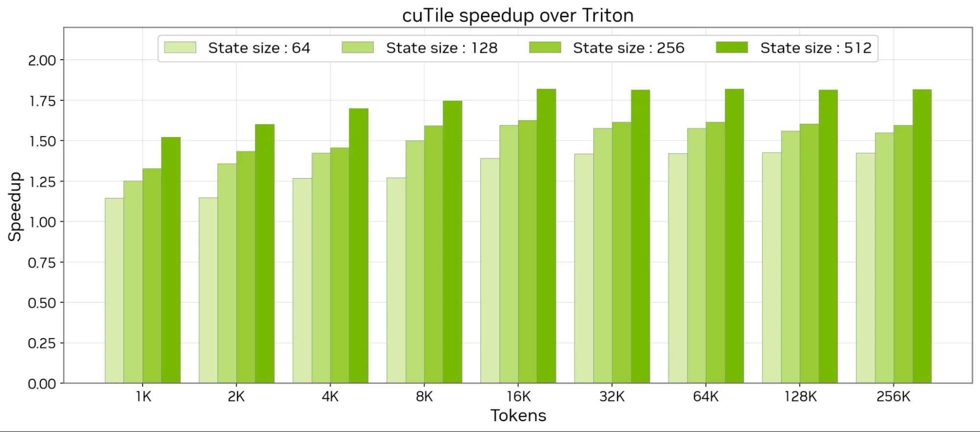 cuTile speedup over the Triton baseline for the Mamba-2 forward pass, by sequence length and state size. Source: NVIDIA.
What the chart shows (values read off the chart):
- cuTile is faster in every configuration tested, from about 1.15× (state size 64, 1K tokens) to about 1.8× (state size 512).
- Bigger states gain more. At every sequence length, the speedup climbs with state size: 64 < 128 < 256 < 512. Larger states mean bigger matmuls, which is where cuTile’s Tensor Core mapping pays off.
- Longer sequences gain more, then level off. Speedups rise from 1K to about 16K tokens, then hold steady out to 256K tokens. At state size 512, the speedup stays around 1.8× across the whole range.