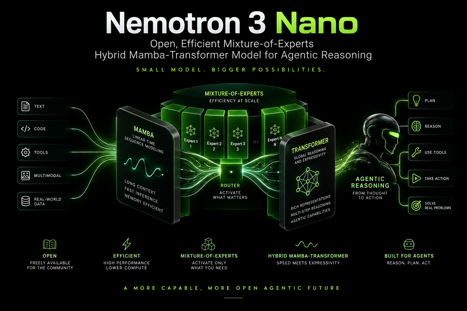
This is an engineering implementation of Nemotron 3 Nano — NVIDIA’s open Mixture-of-Experts (MoE) hybrid Mamba-Transformer model. Rather than summarizing the report, this series reconstructs the system from an engineering and inference standpoint: what the design costs, what it buys, and why the choices matter when you actually have to serve the model.
Source paper: Nemotron 3 Nano: Open, Efficient Mixture-of-Experts Hybrid Mamba-Transformer Model for Agentic Reasoning (NVIDIA, arXiv:2512.20848). This page is the reference/source for the implementation.
What Nemotron 3 Nano Is
Nemotron 3 Nano is an open language model with a specific engineering thesis: you should not have to pay for every parameter on every token. It is a hybrid architecture — Mamba-2 sequence layers and attention interleaved with Mixture-of-Experts layers in place of dense feed-forward networks — trained for reasoning, coding, and agentic workloads rather than short single-turn chat. [Paper]
That workload focus is the framing I carry through the whole series. This is not a general “ARC model” or a new model category; it is an efficient hybrid MoE model whose positioning is long-context reasoning and agentic tasks — tool use, multi-turn interaction, and coding — where a model has to stay cheap while thinking for a long time. [Interpretation]
Why the “A3B” Designation Matters
The model’s full name is Nemotron 3 Nano 30B-A3B, and the two numbers describe two very different quantities.
- 30B is the total parameter count — the full set of weights that live in memory. In practice the model holds ~31.6B total parameters. [Paper]
- A3B means “Active 3B”: roughly 3 billion parameters are active per token, per forward pass. The paper reports ~3.2B active parameters (≈3.6B if you include embeddings). [Paper]
The gap between those two numbers is the entire point of the MoE design. A router selects only a small subset of experts for each token, so the FLOPs and memory bandwidth spent on the forward pass scale with the active parameters, not the total ones. [Interpretation] Concretely, Nemotron 3 Nano activates less than half of its parameters per forward pass while still delivering better accuracy than Nemotron-2 Nano. [Paper]
From an inference perspective this is what you care about: total parameters set your memory footprint, but active parameters set your latency and throughput. A3B is a promise about the second number — you get the capacity of a ~30B model with the per-token compute closer to a ~3B one. [Interpretation]
Why Efficiency, Reasoning, and Long Context Together
Any one of these properties is achievable alone. The engineering interest is in getting all three at once, because that combination is what a real agent needs.
- Efficiency. On a generation-heavy 8K-input / 16K-output scenario, Nemotron 3 Nano reports up to 3.3× higher inference throughput than Qwen3-30B-A3B-Thinking-2507 and about 2.2× higher than GPT-OSS-20B — while being more accurate on popular benchmarks, not just cheaper. [Paper]
- Reasoning. It is trained to think before answering and evaluated on the standard reasoning/thinking suites — for example strong math reasoning on AIME25, coding on SWE-Bench and LiveCodeBench, instruction following on IFBench, and tool use on τ²-Bench. [Paper]
- Scale of training. These capabilities come from pretraining on roughly 25 trillion tokens, including about 3 trillion new tokens added over the Nemotron-2 corpus, followed by supervised fine-tuning and large-scale RL. [Paper]
The reason to state these together is that they are in tension: reasoning models normally cost more at inference because they emit long chains of thought. Nemotron 3 Nano’s claim is that the MoE + hybrid design lets it reason and run fast, which is exactly the trade-off an inference engineer is usually forced to make by hand. [Interpretation]
The 1M-Token Context Window and Agentic Workloads
The capability I want to foreground is the 1 million-token context window. [Paper] For chat this is a nice-to-have; for agentic reasoning and coding, it is close to a requirement.
A long-running agent accumulates state — tool outputs, intermediate reasoning, retrieved files, multi-turn history — and that state grows with every step. A 1M-token window means the agent can keep a large working context resident instead of aggressively summarizing or dropping it, and the paper reports that Nemotron 3 Nano holds up on long-context evaluation (RULER) across context lengths, including at 1M tokens. [Paper]
Pairing that window with the A3B efficiency profile is the combination that matters for long-running agent workflows: long context lets the agent remember, and low per-token cost lets it keep going without the price of a large context making each step prohibitive. [Interpretation]
Accuracy and Throughput at a Glance
The headline comparison is against two similarly-sized open models — Qwen3-30B-A3B-Thinking-2507 and GPT-OSS-20B — across chat, math, instruction following, tool use, coding, and long context, plus a throughput measurement. [Paper]
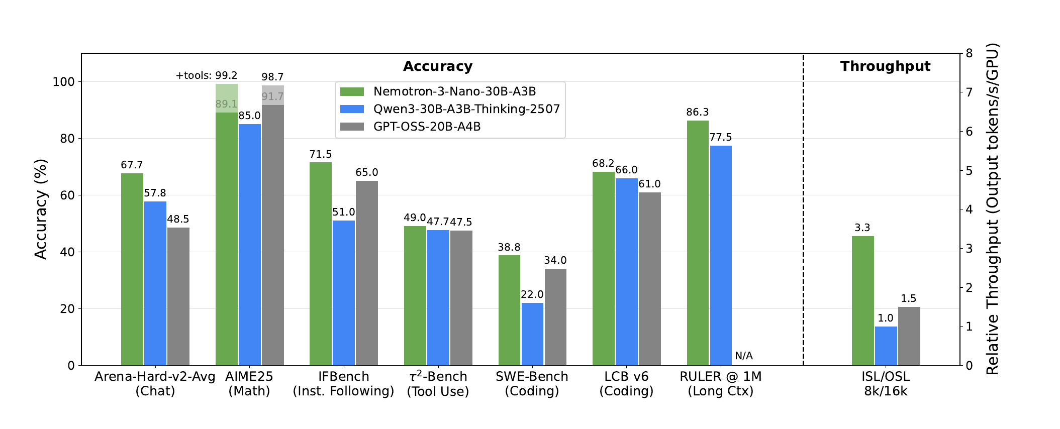
Figure 1 (from the paper) — Accuracy and throughput of Nemotron 3 Nano vs. Qwen3-30B-A3B-Thinking-2507 and GPT-OSS-20B. RULER @ 1M is reported only for Nemotron 3 Nano and Qwen3, because GPT-OSS-20B has a 128K context limit. Throughput is measured on a single H200 GPU with vLLM and TRT-LLM (best of the two per model).
| Benchmark (metric) | Nemotron 3 Nano 30B-A3B | Qwen3-30B-A3B-Thinking-2507 | GPT-OSS-20B-A4B |
|---|---|---|---|
| Arena-Hard-v2-Avg (Chat) | 67.7 | 57.8 | 48.5 |
| AIME25 (Math) | 89.1 (99.2 +tools) | 85.0 | 91.7 (98.7 +tools) |
| IFBench (Inst. Following) | 71.5 | 51.0 | 65.0 |
| τ²-Bench (Tool Use) | 49.0 | 47.7 | 47.5 |
| SWE-Bench (Coding) | 38.8 | 22.0 | 34.0 |
| LCB v6 (Coding) | 68.2 | 66.0 | 61.0 |
| RULER @ 1M (Long Ctx) | 86.3 | 77.5 | N/A |
| Relative throughput (8K in / 16K out) | 3.3× | 1.0× | 1.5× |
The reading I take from this table: Nemotron 3 Nano is at or ahead of both models on almost every axis except raw AIME25 math (where GPT-OSS-20B edges it on the no-tools score), and it does so while generating tokens 3.3× faster than Qwen3 and 2.2× faster than GPT-OSS-20B on the generation-heavy 8K/16K scenario. The long-context result (RULER @ 1M) is one only the 1M-context models can even report. [Interpretation]
Inside the Layer Pattern: Hybrid Mamba-Transformer + MoE
The architecture is a hybrid Mamba-Transformer that scales sparsely: standard feed-forward networks are replaced by Mixture-of-Experts layers, and most of the sequence mixing is done by Mamba-2 layers with attention used only occasionally. [Paper] The paper summarizes this as a repeating layer pattern:
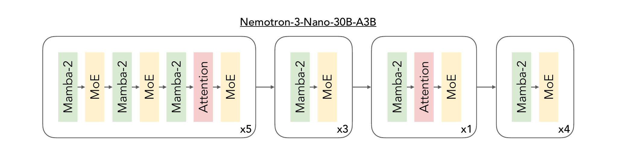
Figure 2 (from the paper) — the Nemotron 3 Nano layer pattern. A hybrid Mamba-Transformer that scales sparsely by using MoE layers instead of standard FFN layers.
Redrawn below as an expanded, per-layer view — each slab is one block, grouped into the four repeating units (×5, ×3, ×1, ×4) that stack into the full 52-layer model. Notice how sparse attention is: it appears only twice in the entire repeating template, while Mamba-2 carries the bulk of sequence mixing and an MoE layer follows almost every mixer. [Interpretation]
All per-block numbers in the legend come from the architecture table below. [Paper]
Architecture Specifications
The full configuration of Nemotron 3 Nano 30B-A3B Base (Table 1 in the paper). [Paper]
| Component | Parameter | Value |
|---|---|---|
| Model | Num Layers | 52 |
| Model Dimension | 2688 | |
| Attention (GQA) | Q-heads | 32 |
| KV-heads | 2 | |
| Head Dimension | 128 | |
| Mamba-2 | State Dimension | 128 |
| Groups | 8 | |
| Heads | 64 | |
| Head Dimension | 64 | |
| MoE | Expert Dimension | 1856 |
| Total Routable Experts | 128 | |
| Activated Experts | 6 | |
| Shared Experts | 2 |
The two KV-heads against 32 query-heads (a 16:1 GQA ratio) and the small Mamba state are both bandwidth choices — they keep the per-token KV and state footprint small, which is what lets throughput stay high while the context window grows toward 1M tokens. [Interpretation]
How Nemotron 3 Nano Was Built (Overview)
This is a high-level map of the training recipe; each stage gets its own deep dive in later parts of this series.
Pretraining. The base model was trained on ~25 trillion tokens of text spanning 15 data categories, using the Warmup-Stable-Decay (WSD) learning-rate schedule. Pretraining ran in two phases: a first phase of ~23.5 trillion tokens of diverse data, followed by a second phase of ~1.5 trillion tokens of high-quality data. [Paper] The resulting base model beats an equivalent-sized Qwen3-30B-A3B-Base on most academic benchmarks across Code, Math, Long Context, General Knowledge, and Commonsense Understanding. (No comparison to GPT-OSS-20B is possible — no base model was released for it.) [Paper]
Post-training. Three stages turn the base model into the released model: [Paper]
- Supervised fine-tuning (SFT) on diverse chat, agentic, and reasoning traces — this is what installs reasoning budget control, reasoning on/off control, and tool-integrated reasoning.
- Multi-environment RL from verifiable rewards (RLVR), trained on all environments simultaneously for a smooth, uniform lift in capabilities.
- RL from human feedback (RLHF), using a large generative reward model (GenRM) to push key chat benchmarks.
Quantization. The model is quantized from bfloat16 to FP8 via post-training quantization (PTQ), which is what buys the higher inference throughput with minimal accuracy loss — and why the released FP8 checkpoint is the one to serve. [Paper]
Model Checkpoints on Hugging Face
The weights, recipe, and most of the training data are released openly. The checkpoints are hosted on Hugging Face under the nvidia organization: [Paper]
 NVIDIA-Nemotron-3-Nano-30B-A3B-FP8 — the final post-trained model, FP8-quantized for inference.
- NVIDIA-Nemotron-3-Nano-30B-A3B-BF16 — the post-trained model in BF16.
- NVIDIA-Nemotron-3-Nano-30B-A3B-Base-BF16 — the pre-trained base model in BF16.
- Qwen3-Nemotron-235B-A22B-GenRM — the generative reward model used for RLHF.
The code is released at NVIDIA-NeMo/Nemotron. [Paper]
Released Datasets
Most of the training data is published as well — the pretraining corpora plus the new SFT and RL collections: [Paper]
- Nemotron-CC-v2.1 — ~2.5T new English tokens from Common Crawl (3 recent snapshots, synthetic rephrasing, translation to English).
- Nemotron-CC-Code-v1 — ~428B high-quality code tokens from Common Crawl Code via the Lynx + LLM pipeline; standardizes math to LaTeX and removes noise.
- Nemotron-CC-Math-v1 — the math pipeline the code corpus builds on.
- Nemotron-Pretraining-Code-v2 — refreshed, curated GitHub code with multi-stage filtering, dedup, and large-scale synthetic code.
- Nemotron-Pretraining-Specialized-v1 — synthetic datasets for specialized areas like STEM reasoning and scientific coding.
- Nemotron-SFT-Data & Nemotron-RL-Data — the new SFT and RL datasets, released under the Nemotron post-training v3 collection.
Attribution convention. Everything below mixes what the paper reports with my own reasoning, so every non-obvious technical claim is tagged:
- [Paper] — stated explicitly in Nemotron 3 Nano (arXiv:2512.20848).
- [Derived] — a mathematical or logical consequence of the paper’s method, worked out here.
- [Interpretation] — my explanation or engineering reasoning, written for the reader; not a claim the paper makes.
- [Background] — established prior work (e.g. the Mamba-2 or attention math) that Nemotron 3 Nano builds on but does not re-derive; I bring it in from the source papers so the mechanism is reconstructable.
The Model Architecture
Hybrid Mamba-Transformer: Why Not Pure Attention or Pure Mamba
Nemotron 3 Nano is a hybrid Mamba-Transformer. It builds directly on the hybrid architecture of NVIDIA’s earlier Nemotron-H and Nemotron 2 Nano, and the one change that defines this generation is replacing the standard feed-forward (FFN) layers with sparse Mixture-of-Experts (MoE) layers. [Paper]
To see why a hybrid is the right call, it helps to remember what each ingredient costs. I walked through the Mamba side of this in detail in the Mamba: Linear-Time Sequence Modeling with Selective State Spaces implementation — that article is the prerequisite here, and I won’t re-derive it. The short version: [Background]
- Attention mixes every token with every other token. That is $O(L^2)$ compute in the sequence length $L$, and — the part that actually hurts at inference — it keeps a KV cache that grows linearly with $L$. At a 1M-token context, the KV cache, not the weights, becomes the thing that blows up your memory budget.
- Mamba-2 is a selective state-space model (SSM). It carries a fixed-size recurrent state and updates it token by token, so it runs in $O(L)$ time with $O(1)$ state per step — no growing cache. The price is that all history has to be compressed into that fixed state, so a pure-SSM model can struggle with tasks that need sharp, exact recall of a specific earlier token.
The hybrid resolves the tension by using each where it is strong: [Interpretation]
- Mamba-2 carries the bulk of sequence mixing. In the repeating layer template it appears far more often than attention, so most of the model’s per-token work is linear-time and cache-free. This is precisely what makes the march toward a 1M-token context affordable.
- Attention appears sparingly — only twice in the entire repeating template (see the layer-pattern diagram above) — to provide the occasional exact, global token-to-token lookup that a pure SSM lacks.
So the architecture is not “attention plus some Mamba”; it is mostly Mamba, punctuated by attention, with MoE doing the channel-wise (per-token) computation in between. [Interpretation]
Dense vs. Sparse: What the MoE Layers Change
The MoE layers are the second half of the efficiency story, and they operate on a different axis than the Mamba/attention choice. Mamba-vs-attention is about how tokens mix across the sequence; dense-vs-sparse is about how much of the network each token flows through.
A dense model — the classic Transformer FFN — sends every token through every parameter of the feed-forward block. If the FFN has $N$ parameters, every token pays for all $N$. Capacity and per-token cost are welded together: the only way to make the model “know more” is to make every token more expensive. [Background]
A sparse MoE model breaks that weld. It replaces the single dense FFN with a pool of smaller expert FFNs plus a router that, per token, selects only a few experts to actually run. [Paper] The total parameter pool can be large (lots of stored knowledge), while the compute per token stays small (only the selected experts fire). Capacity scales with the pool; cost scales with the selection.
A note on framing, because it is easy to overstate: [Interpretation] dense and sparse are architectural choices, not company signatures. It is fair to say “Nemotron 3 Nano is sparse (MoE) whereas a dense model routes every token through the full FFN” — but it is not fair to claim that any given lab (Anthropic, OpenAI, …) uses one approach across all its models. Model families mix and match, and most labs don’t disclose which. The useful comparison is dense FFN vs. sparse MoE as mechanisms, and Nemotron 3 Nano is squarely on the sparse side.
Expert Routing: 128 Experts, 6 Activated, 2 Shared
Nemotron 3 Nano uses a granular MoE with shared experts. Per MoE layer: [Paper]
- 128 total routable experts. These are the pool.
- 6 activated experts per token. A learnt router picks which 6 to run for each token.
- 2 shared experts that run for every token, regardless of routing. Shared experts capture common, always-useful computation so the routed experts can specialize.
- Expert dimension 1856, squared-ReLU activation.
The router itself is a standard learnt MLP router with sigmoid gating. [Paper] It is trained jointly with the rest of the model — the paper describes a single learnt router with sigmoid gating and gives no indication of a separately-trained router, so I make no such claim here. During pretraining, load is balanced with DeepSeek’s auxiliary-loss-free load balancing (update rate $10^{-3}$) in conjunction with the standard load-balancing loss (coefficient $10^{-4}$). [Paper] The aux-loss-free scheme nudges an additive per-expert bias so the router spreads tokens evenly across experts without a strong auxiliary loss fighting the main objective. [Background]
Mechanically, for a token representation $x$ the router produces a score per expert, keeps the top-6, and the layer output is the sum of the 2 shared experts plus the 6 routed experts weighted by their (sigmoid) gates:
\[y = \sum_{s \in \text{shared}} E_s(x) \;+\; \sum_{i \in \text{top-6}} g_i \, E_i(x), \qquad g_i = \sigma(\text{router}(x)_i).\]This is the standard granular-MoE-with-shared-experts formulation from DeepSeek-style MoE; Nemotron 3 Nano adopts it rather than inventing a new router. [Background]
The A3B Arithmetic: Total vs. Active Parameters
This is the number that matters most, and it is the easiest to misread. Two quantities are in play, and they differ by nearly 10×: [Paper]
| Quantity | Value | What it governs |
|---|---|---|
| Total parameters | 31.6B | Memory footprint — every weight must live in GPU memory |
| Active parameters / token | 3.2B (3.6B incl. embeddings) | Compute + bandwidth per forward pass — sets latency and throughput |
The single most important sentence to internalize:
31.6B total parameters ≠ 31.6B parameters used for every token. Only about 3.2B parameters are active per forward pass.
The gap is exactly the MoE effect. Of the 128 routed experts in each MoE layer, only 6 fire per token (plus the 2 shared), so the vast majority of the 31.6B pool sits idle for any given token — different tokens light up different experts. [Interpretation]
A tempting but wrong shortcut. You might try to size a single expert as:
\[\frac{3.2\text{B active}}{6 \text{ activated experts}} \approx 0.53\text{B per selected expert}.\]This 0.53B figure is only a crude average, not the real per-expert parameter count. [Derived] The 3.2B of active parameters is not just the six routed experts — it also includes the 2 shared experts, the Mamba-2 and attention blocks in that layer, the router, RMSNorm, and projections. Dividing the whole active budget by 6 silently attributes all of that to the routed experts and ignores the shared experts entirely. Treat 0.53B as a back-of-envelope sense of scale (“each routed expert is well under a billion parameters”), and never as the exact size of an expert. [Interpretation]
Why This Matters for Inference
The payoff of the whole design shows up at serving time, and it is worth being precise about why: [Interpretation]
- Total parameters set your memory footprint. You still have to store all 31.6B weights (in FP8 for the released checkpoint), so the model occupies the memory of a ~30B model.
- Active parameters set your speed. Each generated token only touches ~3.2B parameters, so the FLOPs and — critically for decode — the memory bandwidth per token are closer to a ~3B model. Autoregressive decoding is bandwidth-bound, and MoE sparsity is a direct cut to bytes moved per token.
- The hybrid keeps the KV cache small. Because attention appears in only 6 of 52 layers and uses a 16:1 GQA ratio (32 query heads sharing 2 KV heads), the KV cache that normally dominates long-context serving stays modest, and the Mamba-2 layers carry no growing cache at all.
Those three effects compound into the headline result: on the generation-heavy 8K-input / 16K-output scenario, on a single H200 with the better of vLLM / TRT-LLM, Nemotron 3 Nano reports up to 3.3× the throughput of Qwen3-30B-A3B-Thinking-2507 and ~2.2× that of GPT-OSS-20B. [Paper]
One caveat, stated plainly: [Interpretation] these multipliers are for that scenario, on that hardware, with those serving stacks. MoE throughput depends on batch size, sequence lengths, expert-parallel layout, and kernel quality; the shape of the win (sparse activation + small cache → faster decode) generalizes, but the exact “3.3×” should not be quoted as a hardware-independent constant.
Inside the Blocks
The layer template stacks three block types. Two of them — Mamba-2 and attention — the paper uses but does not re-derive (it cites Mamba-2 and gives hyperparameters). To keep this reconstructable, I bring the mechanics in from the source work and mark them [Background]; the specific dimensions are [Paper].
Mamba-2, Explained at Three Levels
Nemotron 3 Nano’s Mamba-2 layers use state dimension 128, 8 groups, 64 heads, head dimension 64. [Paper] Here is what those layers actually do, built up in three passes. (Full derivation in the Mamba implementation.) [Background]
Level 1 — the intuition. A Mamba layer is a smart running summary. As it reads the sequence left to right, it keeps a fixed-size memory (the “state”) and, at each token, decides what to write into memory and what to read out. Unlike attention, it never looks back over all previous tokens — it only consults its summary. That is why its cost per token is constant no matter how long the sequence gets.
Level 2 — the recurrence. A state-space model maps an input sequence $x_t$ to outputs $y_t$ through a hidden state $h_t$:
\[h_t = \bar{A}\, h_{t-1} + \bar{B}\, x_t, \qquad y_t = C\, h_t.\]$h_t$ is the fixed-size state (here, 128-dimensional per head). $\bar{A}$ controls how much of the past is retained, $\bar{B}$ how the current input is written in, and $C$ how the state is read out. In a classical SSM these matrices are fixed. Mamba’s key move is selectivity: $\bar{B}$, $C$, and the discretization step $\Delta$ are functions of the input $x_t$, so the model can choose, per token, to remember or forget. That input-dependence is what lets an SSM behave like a content-aware filter instead of a static convolution. [Background]
Level 3 — why Mamba-2 is fast (SSD). Written as a recurrence, the above is inherently sequential — bad for GPUs during training. Mamba-2’s State Space Duality (SSD) restricts $\bar{A}$ to a scalar-times-identity structure, which makes the whole sequence-to-sequence map expressible as a structured matrix multiply. That has two consequences: [Background]
- Training can run as a chunked, parallel scan (matmuls the hardware loves) instead of a token-by-token loop.
- There is a formal duality with attention — the SSM can be viewed as a form of linear attention with a decay structure — which is why a hybrid with real attention slots together so cleanly conceptually.
The 8 groups are the SSM analogue of GQA’s KV sharing: parameters like $\bar{B}$/$C$ are shared across heads in a group to cut state size and bandwidth, while the 64 heads give the layer enough independent channels to be expressive. [Interpretation]
The Attention Blocks: Grouped-Query Attention
The two attention layers use Grouped-Query Attention (GQA) with 32 query heads, 2 KV heads, head dimension 128, and — notably — no positional embeddings (the Mamba layers supply order information), RMSNorm for normalization, and no bias on linear layers. [Paper]
Standard attention computes, per head:
\[\text{Attn}(Q,K,V) = \text{softmax}\!\left( \frac{QK^\top}{\sqrt{d_k}} \right) V.\]The expensive part at inference is not the matmul — it is storing $K$ and $V$ for every past token (the KV cache). GQA shrinks that cache by letting several query heads share one key/value head. [Background] With 32 query heads mapped onto 2 KV heads, the KV cache is 16× smaller than full multi-head attention would need, for nearly the same quality. [Derived] Combined with attention appearing in only 6 of 52 layers, this is what keeps long-context serving tractable. [Interpretation]
Tracing One Token Through a Layer
Putting the blocks together, here is the path a single token’s representation $x$ takes through the repeating template, so the data flow is concrete: [Interpretation]
- RMSNorm normalizes $x$.
- It enters the sequence mixer — usually a Mamba-2 layer (state updated, output read out), occasionally an attention layer (query against the small GQA KV cache).
- A residual add returns to the stream; another RMSNorm precedes the channel mixer.
- The MoE layer routes $x$: the sigmoid-gated router scores all 128 experts, the top-6 run and are combined by their gates, the 2 shared experts always run, and the results sum.
- A final residual add, and the token moves to the next block.
Across 52 layers this repeats, with the group pattern (×5, ×3, ×1, ×4 from the diagram) fixing where the two attention layers land. [Paper]
Pre-training
The Data: Four New Corpora
The base model was trained on ~25 trillion tokens, adding more than 3 trillion new unique tokens over the Nemotron 2 corpus. [Paper] The genuinely new pretraining data is released as four datasets: [Paper]
- Nemotron-CC-Code-v1 — ~427.9B code tokens. Code pages from Common Crawl, rendered with Lynx to preserve indentation, cleaned by Phi-4, and filtered by a code-quality classifier. Equations are standardized to LaTeX and code blocks kept structurally intact.
- Nemotron-Pretraining-Code-v2 — refreshed GitHub code. New repos (cutoff April 15, 2025), deduplicated against the existing corpus, plus synthetic code: Qwen3-32B-generated Q&A and student-teacher/code-review dialogues, SGCR/SCOR rephrasing of Python source, and Python→C++ transpilation (which improved downstream C++ accuracy).
- Nemotron-CC-v2.1 — >2.5T new English tokens. Three fresh Common Crawl snapshots on the Nemotron-CC recipe; rephrasing prompts applied to Medium-High-Quality data across 110 snapshots (2.1T new tokens); and a novel translate-to-English path from 9 languages, quality-filtered. A late LLM quality pass removed ~10.6% of tokens in the released version.
- Nemotron-Pretraining-Specialized-v1 — synthetic specialized data. Synthetic Wikipedia, synthetic math-textbook sections, synthetic scientific coding, a cross-domain InfiniByte code generator, and a Reasoning QA (RQA) set — 4.3M demonstrations, ~31.7B tokens — plus a diverse-QA (DQA) set (~8B tokens).
Additional refreshed SFT-style data (math, code, STEM) was also folded into pretraining, with responses from DeepSeek-R1. [Paper]
Data Mixture and Two-Phase Curriculum
The corpus spans fifteen data categories. [Paper] The largest is web crawl, subdivided into five quality buckets following the Nemotron-CC taxonomy (crawl-medium, crawl-medium-high, syn-crawl-medium-high, crawl-high, syn-crawl-high). Beyond crawl, the mixture includes math, Wikipedia, code, nemotron-cc-code, academic text, Crawl++ (OpenWebText, BigScience, Reddit), multilingual data (19 languages), and synthetic SFT-style data grouped into general-sft, stem-sft, and code-sft. [Paper]
Training used a two-phase curriculum, switching phases at the 94% point of training: [Paper]
- Phase 1 (first ~94%) — a diversity-promoting mixture, drawing broadly across all categories.
- Phase 2 (final ~6%) — primarily high-quality data (e.g. Wikipedia), with the synthetic-SFT, math, and STEM shares up-weighted relative to Phase 1. [Paper] (Exact per-category percentages are given in the paper’s Figure 3; I describe the direction of the shift rather than re-transcribe the pie charts, to avoid introducing transcription error into the numbers.) [Interpretation]
Hyperparameters
Pretraining used the Warmup-Stable-Decay (WSD) learning-rate schedule over the full 25T tokens: [Paper]
| Setting | Value |
|---|---|
| LR schedule | Warmup-Stable-Decay (WSD) |
| Warmup | 8.4B tokens → max LR $10^{-3}$ |
| Stable | max LR held for 80% of training (20T tokens) |
| Decay | to min LR $10^{-5}$ over the final 20% (5T tokens) |
| Optimizer | AdamW, weight decay 0.1, $\beta_1=0.9$, $\beta_2=0.95$ |
| Sequence length | 8192 |
| Batch size | 3072 sequences (≈25M tokens/batch) |
| MoE load balancing | aux-loss-free (update rate $10^{-3}$) + standard LB loss (coeff $10^{-4}$) |
Long-Context Extension
After the main run, a long-context phase (LC-Phase) does continuous pretraining (CPT) to push the usable context toward 1M tokens, using 121B tokens total. [Paper] Constant LR $10^{-5}$, global batch size 48, and a heavy parallelism layout on H100s (8-way context / 8-way tensor / 8-way expert / 4-way pipeline parallelism). The blend is 20% long document-QA (reused from Nemotron 2, scaled 3×), 1% synthetic retrieval data (up to 256k tokens), and 79% down-scaled Phase-2 data. Training on pure 512k sequences hurt short-context scores, so a mix of 512k and 4k sequences was used — which recovered short-context benchmarks (notably MMLU-Pro and Code) while still improving long-context ones. [Paper]
Base Model Evaluations
The base model is compared against Qwen3-30B-A3B-Base (no base model exists for GPT-OSS-20B). [Paper] Best per row in bold.
| Task (metric) | Qwen3-30B-A3B-Base | Nemotron 3 Nano 30B-A3B Base |
|---|---|---|
| General Knowledge | ||
| MMLU (5-shot, acc) | 81.07 | 78.56 |
| MMLU-Pro (5-shot, CoT EM) | 61.71 | 65.05 |
| AGIEval-En (3/5-shot, CoT) | 63.12 | 68.32 |
| Code | ||
| HumanEval (0-shot) | 70.73 | 78.05 |
| MBPP-Sanitized (3-shot) | 73.15 | 75.49 |
| Math | ||
| GSM8K (8-shot) | 89.01 | 92.34 |
| MATH (4-shot) | 61.14 | 82.88 |
| MATH-500 (4-shot, avg@32) | 55.08 | 78.63 |
| Commonsense | ||
| ARC-Challenge (25-shot) | 94.45 | 91.89 |
| HellaSwag (10-shot) | 83.14 | 85.56 |
| OpenBookQA (0-shot) | 44.80 | 46.20 |
| PIQA (0-shot) | 81.01 | 84.33 |
| WinoGrande (5-shot) | 78.22 | 79.64 |
| Reading Comp. | ||
| RACE (0-shot) | 90.05 | 88.04 |
| Multilingual | ||
| MMLU Global Lite (5-shot) | 76.84 | 74.47 |
| MGSM (8-shot) | 82.53 | 83.00 |
| Long Context | ||
| RULER @ 64K | 63.55 | 87.50 |
| RULER @ 128K | 60.69 | 82.92 |
| RULER @ 256K | — | 75.44 |
The pattern I read: Nemotron 3 Nano’s base model trades a little raw knowledge breadth (MMLU, ARC-Challenge, multilingual MMLU) for large gains in math (MATH 61→83), code, and — most dramatically — long context, where the hybrid’s linear-time layers let RULER stay strong to 256K while Qwen3’s numbers fall off and aren’t even reported past 128K. [Interpretation]
Post-Training
Post-training scales up compute substantially versus Nemotron 2 Nano, and it is NVIDIA’s first large-scale multi-environment RL effort — training on all RL environments simultaneously. The pipeline has a specific order, which is worth stating exactly because it is easy to get wrong: [Paper]
\[\textbf{SFT} \;\rightarrow\; \textbf{RLVR}_1 \;\rightarrow\; \textbf{RLHF} \;\rightarrow\; \textbf{RLVR}_2.\]Two stages of RLVR bracket the RLHF stage — one immediately after SFT, one after RLHF. [Paper] Tooling: NeMo Gym (environment orchestration) integrated with NeMo RL (training loop, on Megatron-Core), both open-sourced. [Paper]
Stage 1 — Supervised Fine-Tuning (SFT)
SFT installs the model’s behaviors: chat formatting, tool use, reasoning control, and domain skills. Unlike the pretraining SFT-style data, this stage applies the chat template and leans heavily on multi-step, multi-turn agentic tasks. [Paper]
Chat template and reasoning flow. The template supports reasoning and non-reasoning modes. In multi-step (a chain of assistant calls) the existing reasoning is preserved for reuse; in multi-turn (a new user message) reasoning from previous turns is dropped — for any generation, only the current turn’s reasoning is materialized into the prompt. Tool calls use XML-style tags to reduce escaping. [Paper]
Data domains. The SFT data spans competition math (refreshed with GPT-OSS-120B, plus tool-integrated Python reasoning traces), competition code, conversational tool use (LLM-judge-filtered synthetic trajectories), long context (mean 128k / max 256k tokens), formal proofs (Lean 4 — 580k autoformalized theorems → 550k statements → Goedel-Prover-V2-32B proof generation → 300k compiler-verified examples), multilingual, terminal use (Terminal-Bench-style, SWE-Smith), general chat, instruction following (Tülu-3 methodology, IFEval/IFBench-verified), safety, software engineering (SWE-Gym / R2E-Gym issues, distilled from OpenHands / SWE-Agent / Mini-SWE-Agent), science (physics/chemistry/biology MCQ→OpenQA), GenSelect (best-of-N selection traces), and CUDA (21k PyTorch↔CUDA-C pairs, compiled and numerically verified). [Paper]
SFT data blend (Figure 5, ~18M total samples). Datasets under 1% are omitted. [Paper]
| Domain | Share | Domain | Share |
|---|---|---|---|
| Chat | 28.6% | Math w/ Tools | 4.9% |
| Code | 20.7% | GenSelect | 3.0% |
| Science | 12.8% | SWE | 3.0% |
| Math | 9.9% | Formal Proofs | 2.0% |
| Multilingual | 7.4% | Long Context | 2.0% |
| Conversational Agent | 2.0% | Terminal Use | 1.5% |
Data filtering. A unified pipeline drops malformed examples (e.g. tool calls without tool definitions), aggressively removes traces with pathological n-gram repetition, and applies keyword/regex filters to strip trajectories that drift into nationalistic or politically-aligned narratives. [Paper]
Reasoning control. Two controls are baked in during SFT: reasoning on/off (strip the reasoning trace from a random 10% of samples) and token-budget control (randomly truncate reasoning in 3% of samples to varying budgets, then continue with the original post-reasoning answer). [Paper] This is what lets a downstream agent say “think hard” or “answer immediately” without a different model.
SFT hyperparameters. 13,000 steps, batch size 64, sequence packing to length 256K, LR $5\times10^{-5}$ with 800 warmup steps, sequence-level MoE load-balancing regularizer (coeff $10^{-4}$). [Paper]
Stage 2 & 4 — RLVR (Reinforcement Learning from Verifiable Rewards)
A note on naming/fidelity: the paper’s term is RLVR — Reinforcement Learning from Verifiable Rewards (§3.2). There is no stage called “SLVR”. I use RLVR throughout. [Interpretation]
RLVR trains against verifiable reward signals — unit tests, exact schema matches, database-state checks, LLM-judge verifiers — across many environments at once, which the paper finds gives stable, uniform gains where single-environment training tends to degrade other skills. [Paper]
Environments (task counts): competition math (DAPO 17K + SkyWorks 104K), competition coding (22K, ≤50 unit tests each), STEM question-answering (135K), structured outputs / JSON-schema adherence (9K, exact-match reward), instruction following (IFBench-style 46K + multi-turn LLM-judge 3K), long context (12K, ≥5-document QA within 32k tokens), and agentic tool use (Workplace Assistant: 5 databases / 26 tools / 690 tasks; plus a multi-turn banking agent, ~1K tasks). [Paper]
Curriculum. Tasks are first profiled with the SFT checkpoint; anything the SFT model already solves at 100% pass rate is filtered out. Difficulty is then scheduled via a Gaussian target-pass-rate whose mean decreases linearly over training — easy early, hard late — with fixed per-domain ratios in each batch. The paper shows this beats random sampling, which biases toward easy tasks. [Paper]
Does RL actually beat a strong SFT model? To test this, the paper compares RLVR against two SFT checkpoints: SFT1 (~3 epochs) and SFT2 (fully converged, ~5 epochs). [Paper] Even with short training, RLVR matches or exceeds the heavily-converged SFT2 across every evaluated domain. Note these are ablation checkpoints demonstrating RL’s value — not sequential pipeline stages, and there is no “CCB1” checkpoint anywhere in the recipe. [Interpretation]
Algorithm. Synchronous GRPO with masked importance sampling (to mitigate train/inference mismatch): 128 prompts/step, 16 generations/prompt, batch 2048 (on-policy updates), MoE router weights frozen, aux-loss-free load balancing with expert-bias updates kept on, max generation length 49K, and overlong filtering (which helps reasoning-heavy benchmarks). [Paper]
Stage 3 — RLHF with a Generative Reward Model
RLHF pushes chat quality using a generative reward model (GenRM) rather than a classic Bradley-Terry scalar model — GenRMs generalize better and resist reward hacking. [Paper] The GenRM is a fine-tuned Qwen3-235B-A22B-Thinking-2507 (released as Qwen3-Nemotron-235B-A22B-GenRM), trained with GRPO to reason over two candidate responses and emit helpfulness scores ($1$–$5$ each) plus a ranking score ($1$–$6$). [Paper]
GenRM reward. Training reward for the GenRM: [Paper]
\[R = -C_1 I_{\text{format}} - |P_{h1}-G_{h1}| - |P_{h2}-G_{h2}| - C_2\,|P_r - G_r|, \qquad C_1=10,\; C_2=1,\]where $P$/$G$ are predicted/ground-truth helpfulness ($h1,h2$) and ranking ($r$) scores, and $I_{\text{format}}$ flags a format violation. Intuitively: match the human helpfulness and ranking labels, with a heavy penalty for malformed output. Each sample is also position-swapped to kill positional bias.
Scaling comparisons cheaply. During RLHF (same 128 prompts × 16 responses as RLVR), naively scoring all response pairs is $\binom{N}{2}=120$ GenRM calls per prompt at $N=16$. Instead a circular comparison compares each response only with its successor — $(r_1,r_2),(r_2,r_3),\dots,(r_N,r_1)$ — giving exactly $N$ comparisons and cutting cost from $O(N^2)$ to $O(N)$ while still connecting all responses; each is judged twice in different positions. [Paper] On a tie ($s_i = s_j$) a small tiebreaker uses the ranking score:
\[s_i = s_i + (3.5 - s_r), \qquad s_j = s_j + (s_r - 3.5).\]Group Relative Length Control. A base reward built from these comparisons causes response length to balloon (mostly reasoning tokens, even though only the final answer is judged). To stop that without penalizing genuinely hard prompts, the paper adds a zero-mean, group-relative length bonus. Reasoning lengths are normalized within the group of $N$ candidates: [Paper]
\[w_i^{(\text{think})} = 1 - \frac{\ell_i^{(\text{think})} - \ell_{\min}^{(\text{think})}}{\ell_{\max}^{(\text{think})} - \ell_{\min}^{(\text{think})}},\]then centered so the adjustment is zero-sum across the group (preserving overall reward scale):
\[\tilde{w}_i^{(\text{think})} = w_i^{(\text{think})} - \frac{1}{N}\sum_{j=1}^{N} w_j^{(\text{think})}.\]The same is done for answer length, and the final per-response reward is:
\[R_i = R_i^{(\text{base})} + \lambda^{(\text{think})}\,\tilde{w}_i^{(\text{think})} + \lambda^{(\text{answer})}\,\tilde{w}_i^{(\text{answer})}, \qquad \lambda^{(\text{think})}=\lambda^{(\text{answer})}=0.5.\]A quality-gated conciseness bonus then adds $\beta=0.5$ to the shortest reasoning/answer responses only if their base reward clears the group’s $p=80$th-percentile threshold $\tau_p$ — so shortness is rewarded only when quality is already top-tier. Net effect: ~30% less verbosity with no accuracy loss. [Paper] Because the penalty is relative within each prompt group, inherently complex prompts are not unfairly punished. [Interpretation]
Post-Trained Model Evaluations
The final model versus Qwen3-30B-A3B-Thinking-2507 and GPT-OSS-20B. [Paper] (* = value from ArtificialAnalysis or computed with the official protocol; — = not reported.)
| Benchmark | N-3-Nano | Qwen3 | GPT-OSS |
|---|---|---|---|
| General Knowledge | |||
| MMLU-Pro | 78.30 | 80.90 | 75.00 |
| Reasoning | |||
| AIME25 (no tools) | 89.06 | 85.00 | 91.70 |
| AIME25 (with tools) | 99.17 | — | 98.70 |
| GPQA (no tools) | 73.04 | 73.40 | 71.50 |
| GPQA (with tools) | 75.00 | — | 74.20 |
| LiveCodeBench v6 | 68.25 | 66.00 | 61.00 |
| SciCode (subtask) | 33.28 | 33.00 | 34.00 |
| HLE (no tools) | 10.57 | 9.80 | 10.90 |
| HLE (with tools) | 15.48 | — | 17.30 |
| MiniF2F pass@1 | 50.03 | 5.72* | 12.05* |
| MiniF2F pass@32 | 79.92 | 16.80* | 43.03* |
| Agentic | |||
| Terminal Bench (hard) | 8.51 | 5.00 | 10.00 |
| SWE-Bench (OpenHands) | 38.76 | 22.00* | 34.00* |
| τ²-Bench (Average) | 49.04 | 47.70 | 47.50 |
| BFCL v4 | 53.76 | 46.40* | — |
| Chat & Instruction Following | |||
| IFBench (prompt) | 71.51 | 51.00 | 65.00 |
| Scale AI Multi-Challenge | 38.45 | 44.75 | 33.75 |
| Arena-Hard-V2 (Average) | 67.65 | 57.80 | 48.55 |
| Long Context | |||
| AA-LCR | 35.85 | 59.00 | 34.00 |
| RULER-100 @ 256k | 92.92 | 89.40 | — |
| RULER-100 @ 512K | 91.25 | 84.00 | — |
| RULER-100 @ 1M | 86.34 | 77.50 | — |
| Multilingual | |||
| MMLU-ProX | 59.50 | 77.60* | 69.10* |
| WMT24++ (en→xx) | 86.20 | 85.60 | 83.20 |
The takeaway the paper draws — and the table supports — is that Nemotron 3 Nano leads clearly in agentic (SWE-Bench, τ²-Bench, BFCL), chat/instruction-following (IFBench, Arena-Hard-V2), formal proofs (MiniF2F, by a wide margin), and long context (RULER at 256k–1M), while staying competitive with GPT-OSS on raw reasoning and trailing on a few knowledge/multilingual rows (MMLU-Pro, MMLU-ProX, AA-LCR). [Interpretation]
Quantization: Selective PTQ to FP8
The released serving checkpoint is FP8, produced by post-training quantization (PTQ) of the BF16 model with ModelOpt + Megatron-LM. [Paper] The design goal is throughput without accuracy loss, and the key idea is that not all layers tolerate quantization equally.
Selective strategy. A sensitivity analysis found the self-attention layers (6 of 52) are the most fragile, so they stay in BF16 — and the Mamba layers that feed into them (another 6) are sensitive too and also stay BF16. Everything else — weights, activations, and the KV cache — is quantized to FP8. The Conv1D inside every Mamba layer stays BF16. [Paper] Calibration used just 1K samples from the reasoning SFT data (better recovery than cnn_dailymail; on-policy calibration gave no benefit). [Paper]
Accuracy vs. BF16 (Table 4) — ~99% median recovery. [Paper]
| Benchmark | BF16 | FP8 |
|---|---|---|
| MMLU-Pro | 78.30 | 78.10 |
| AIME25 (no tools) | 89.06 | 87.71 |
| AIME25 (with tools) | 99.17 | 98.80 |
| GPQA (no tools) | 73.04 | 72.47 |
| GPQA (with tools) | 75.00 | 73.40 |
| LiveCodeBench v6 | 68.25 | 67.62 |
| SciCode | 33.28 | 31.88 |
| HLE (no tools) | 10.57 | 10.33 |
| HLE (with tools) | 15.48 | 14.27 |
| τ²-Bench (Average) | 49.04 | 47.04 |
| BFCL v4 | 53.76 | 53.15 |
| IFBench (prompt) | 71.51 | 72.19 |
| AA-LCR | 35.85 | 36.06 |
| MMLU-ProX | 59.50 | 59.63 |
The interesting engineering result (Figure 11 in the paper): FP8 KV-cache quantization is what actually moves throughput, because a smaller cache lets you run larger batches — and the selective strategy is what lets you quantize the KV cache without the accuracy hit that hits naive full-FP8 configurations. That is why the selective config sits at the top-right (high accuracy recovery and high throughput) of the trade-off curve. [Paper] A couple of rows (IFBench, AA-LCR, MMLU-ProX) even tick up in FP8, which is within evaluation noise, not a real gain. [Interpretation]
The End-to-End Pipeline
Assembling every stage into one view — from raw tokens to the served FP8 checkpoint: [Paper]
                         PRE-TRAINING (base model)
  25T tokens ──> WSD schedule (8.4B warmup → 10⁻³, 80% stable, decay 10⁻⁵)
             ──> two-phase curriculum (switch @ 94%)
             ──> LC-Phase CPT (121B tokens, 512k+4k mix)  ──►  Base 30B-A3B (BF16)
                                                                     │
                         POST-TRAINING                               ▼
        SFT (13k steps, chat template, reasoning control, ~18M samples)
                                                                     │
                                                                     ▼
        RLVR₁  (multi-env GRPO, verifiable rewards, curriculum)
                                                                     │
                                                                     ▼
        RLHF   (GenRM + circular comparison + Group Relative Length Control)
                                                                     │
                                                                     ▼
        RLVR₂  (second verifiable-reward stage)          ──►  Post-trained 30B-A3B (BF16)
                                                                     │
                         QUANTIZATION                                ▼
        Selective PTQ  (keep 6 attn + 6 preceding Mamba in BF16;
                        weights/activations/KV → FP8)     ──►  Nemotron 3 Nano 30B-A3B (FP8)
                                                                (the checkpoint you serve)
Where the Paper and This Walkthrough Differ
In the spirit of strict source fidelity, here is exactly where I departed from a literal transcription, and why: [Interpretation]
- The Mamba-2 and attention equations are
[Background], not[Paper]. The Nemotron 3 Nano report uses Mamba-2 and GQA and gives their hyperparameters, but does not re-derive their math. I brought the mechanics in from the Mamba-2 and attention literature (and my own Mamba implementation) so the blocks are reconstructable. Every dimension (state 128, 8 groups, 32:2 heads, etc.) is[Paper]; the derivations are not. - The pipeline is
SFT → RLVR₁ → RLHF → RLVR₂. There is no “CCB1” checkpoint in the paper. The only named SFT checkpoints are SFT1 (~3 epochs) and SFT2 (~5 epochs), and they are ablation points used to show RLVR beats a converged SFT model — not stages of the recipe. - The reward-model stage is
RLHFwith aGenRM, and the verifiable-reward stages areRLVR. The paper never uses “SLVR”; that spelling does not appear. - Pretraining data-mixture percentages (Figure 3) are described directionally, not tabulated. The per-phase pie-chart values were not transcribed into an exact table here, to avoid introducing OCR/transcription error into numbers the fidelity rules require me to preserve exactly. All other tables (base evals, post-trained evals, FP8 vs BF16, SFT blend) reproduce the paper’s exact numbers.
All quantitative claims above are traceable to Nemotron 3 Nano (arXiv:2512.20848); tags mark where interpretation begins.