This is an engineering dissection of FlashInfer — a customizable, block-sparse attention engine for LLM inference serving. These are my own understanding notes, promoted into an implementation walkthrough: the goal is to go from paper concept → my understanding → engineering interpretation → data/control flow → CUDA/C++ → GPU behavior, so that by the end the reader can reconstruct not just what FlashInfer proposes but how the idea becomes an actual kernel running on an SM.
FlashInfer is the layer underneath a serving system. It has been integrated into vLLM, SGLang, and MLC-Engine, and can act as an attention backend inside TensorRT-LLM. It does not own the model, the requests, or the KV-cache policy — it owns attention execution. Holding that boundary straight is half of understanding the paper, so I keep returning to it.
Attribution convention. Because this mixes what the paper states with my own reasoning and teaching code, non-obvious claims are tagged:
- [Paper] — stated in the FlashInfer paper (§ references are to the paper’s sections/figures).
- [Interpretation] — my engineering reasoning, written for the reader.
- [Educational] — a worked example or representative kernel written here to build intuition; not a verbatim FlashInfer source listing.
- [Explanatory CUDA] — general CUDA/GPU knowledge used to ground something the paper assumes, not something the paper specifies.
Where my explanation and the paper’s framing diverge, I keep my explanation and make the distinction explicit rather than silently rewriting it.
I. The One Distinction That Matters Most: Engine, Not Kernel
Before anything technical, the single idea that everything else hangs off. FlashInfer is not changing the Transformer architecture, and it is not replacing the attention mechanism mathematically. The model still does exactly what it always did:
Q, K, V → attention scores → softmax / variant → weighted V → output
What FlashInfer changes is how that attention computation is implemented on the GPU. [Interpretation]
LLM / Transformer
       │
       ▼
   Attention
       │
       │  "I need attention(Q, KV-cache)"
       ▼
 ┌─────────────────┐
 │    FlashInfer   │
 │                 │
 │ KV-cache layout │
 │ GPU kernel      │
 │ scheduling      │
 │ memory movement │
 └─────────────────┘
       │
       ▼
   Attention output
So for Llama, Qwen, DeepSeek, etc., the model’s attention concept has not fundamentally changed. The backend executing attention has. This is also why the paper’s title says “Attention Engine” rather than “new attention architecture.” [Paper]
Why serving needs an engine and training got by with a kernel
The setup from the paper’s introduction: in LLM serving, the attention mechanism reads from the KV cache (the stored historical context) and computes outputs based on the current query. The efficiency of this attention operator is paramount to overall inference performance. But creating high-performance attention kernels tailored for serving introduces challenges not encountered in training. [Paper]
That third point is the hinge of the whole paper. The attention math is the same as in training, but the serving setting is different: [Interpretation]
        Training                         Serving
   ─────────────────────           ─────────────────────
   fixed, known shapes             query = "now", KV = all history
   uniform sequence lengths        wildly varying lengths per request
   contiguous tensors              paged / shared / reused KV cache
   one static kernel is fine       one static kernel is not enough
So the problem statement isn’t “attention is slow.” It’s: attention in serving is performance-critical and its shapes, layouts, and variants are far less predictable than in training — which is precisely why a kernel isn’t enough and an engine is needed.
Scope check: FlashInfer does not own the Q/K/V projections
“FlashInfer implements attention on the GPU” can be read too widely. The Q, K, V projections are plain matrix multiplications against the learned weights:
\[Q = X W_Q, \qquad K = X W_K, \qquad V = X W_V\]Those are ordinary linear layers. FlashInfer is concerned with the attention computation after the Q/K/V tensors already exist — specifically, efficient attention over the KV cache. [Paper] The mental model is not “FlashInfer → computes QKV projections.” It is:
Input
  │
  ├── Q projection ──► Q
  ├── K projection ──► K ──► KV Cache
  └── V projection ──► V ──► KV Cache
                              │
                              ▼
                         FlashInfer
                              │
                    Attention(Q, K_cache, V_cache)
                              │
                              ▼
                           Output
The four contributions, and where each lives in this article
The paper’s formal contribution list, mapped onto the sections below: [Paper]
| Contribution | Paper section | Where here |
|---|---|---|
| Block-sparse and composable formats for KV-cache heterogeneity | §3.1 | IV |
| Customizable attention template + JIT compilation | §3.2 | VI, VII |
| Dynamic scheduling framework, CUDAGraph-compatible | §3.3 | VIII |
| Comprehensive evaluation | §4 | XI |
One word in that first bullet is easy to skim past: composable. It is not a synonym for block-sparse — it is the second half of the format story, and it is what makes splitting a long KV sequence into chunks and merging the partial results exact rather than approximate. That merge is the ⊕ operator of Section III, so I have to establish ⊕ before the format work makes sense.
II. Background: The Attention Math FlashInfer Inherits
FlashInfer builds on FlashAttention. To understand what FlashInfer adds, I first have to be clear about what it inherits and therefore does not re-invent.
II.1 What FlashAttention solves
Textbook attention materializes the score matrix: [Interpretation]
S = Q Kᵀ          →  write  S  to global memory   (l_qo × l_kv)
P = softmax(S)    →  read S, write P to global memory
O = P V           →  read P
For sequence length n, S and P are n × n. Two problems:
- Memory: O(n²) global memory, purely for intermediates that get thrown away.
- Bandwidth: the matrix is written to HBM and read back repeatedly. Attention is memory-bandwidth bound, not compute bound — the GPU sits waiting on HBM while the Tensor Cores idle.
The key realisation is that this is not a FLOP problem. The arithmetic is unavoidable; the data movement isn’t. FlashAttention is an IO-aware algorithm: same math, far fewer trips to HBM. During the forward pass it employs the online-softmax trick, updating attention outputs on-the-fly using a constant amount of on-chip memory, thus avoiding materializing the attention matrix in global memory. [Paper]
II.2 The online-softmax recurrence
The obstacle to fusing everything into one pass is that softmax appears to need the whole row before it can normalise (you need the row max for stability and the row sum to divide by). Online softmax removes that dependency by carrying running statistics and retroactively rescaling what’s already accumulated. Per tile of K/V, maintaining a running max m and running sum l: [Interpretation]
m_i = max(m_{i-1}, rowmax(S_i))

l_i = e^(m_{i-1} - m_i) · l_{i-1}  +  rowsum(e^(S_i - m_i))
      └──── rescale old ────┘         └──── add new ────┘

O_i = e^(m_{i-1} - m_i) · O_{i-1}  +  e^(S_i - m_i) · V_i
      └──── rescale old ────┘         └─── add new ───┘
When a later tile reveals a larger max, the previously accumulated output is simply scaled by e^(m_old − m_new) to correct it. So the result is exact — not an approximation, not a sparse or low-rank shortcut. That’s why the paper stresses the word exact. The loop:
for each block of Q:                 ← stays in on-chip SRAM
    for each block of K, V:          ← streamed in, one tile at a time
        S_ij = Q_i K_jᵀ              ← computed in SRAM, never written to HBM
        update m, l, O               ← running stats, constant memory
    write O_i to HBM                 ← one write per Q block, that's it
I flag this recurrence now because it is exactly the machinery that makes chunked KV + partial outputs viable in Section III: if you can rescale-and-merge across tiles inside one kernel, you can also rescale-and-merge across CTAs. Same trick, wider scope. [Interpretation]
II.3 Operational intensity — the quantitative reason decode is memory-bound
This is where the paper stops describing FlashAttention and starts explaining why serving is the hard case. Its claim: the operational intensity of FlashAttention is [Paper]
\[O\!\left(\frac{1}{\dfrac{1}{l_{qo}} + \dfrac{1}{l_{kv}}}\right)\]where $l_{qo}$ is the query length and $l_{kv}$ the KV-cache length. Operational (arithmetic) intensity is
\[\text{intensity} = \frac{\text{FLOPs performed}}{\text{bytes moved from memory}}\]Low intensity means memory-bound — starved waiting on HBM, Tensor Cores idle. High intensity means compute-bound, which is where you want to be.
That expression is the harmonic mean of $l_{qo}$ and $l_{kv}$, up to a factor of 2: [Interpretation]
\[\frac{1}{\dfrac{1}{l_{qo}} + \dfrac{1}{l_{kv}}} = \frac{l_{qo}\, l_{kv}}{l_{qo} + l_{kv}}\]The important property of that form is that it is dominated by the smaller of the two. Let $l_{kv} \to \infty$ with $l_{qo}$ fixed:
\[\lim_{l_{kv} \to \infty} \frac{l_{qo}\, l_{kv}}{l_{qo} + l_{kv}} = l_{qo}\]So no matter how enormous the KV cache grows, the intensity saturates at $l_{qo}$. Growing history buys you nothing. And in serving, query length is either equal to the KV length (prefill) or smaller (decode) — never larger. So $\min(l_{qo}, l_{kv}) = l_{qo}$ always, and the intensity simplifies to $O(l_{qo})$. Substitute the decode case, where exactly one token is generated ($l_{qo}=1$):
\[O(l_{qo}) = O(1)\]That single line is the whole reason this paper exists. Constant operational intensity: you stream the entire KV cache out of HBM and do a constant amount of arithmetic per byte loaded.
prefill:  l_qo = l_kv = n     →  intensity O(n)     →  compute-bound, Tensor Cores fed
decode:   l_qo = 1            →  intensity O(1)     →  memory-bound, HBM is the wall
II.4 Why batching does not rescue decode, but GQA does
Batching is the standard fix for memory-bound GPU work everywhere else, and the paper states flatly that it does not alter attention’s operational intensity. The distinction is what gets shared across the batch: [Paper]
| Operation | Batched over B requests | Shared data? | Effect on intensity |
|---|---|---|---|
| Linear layer ($XW$) | $B$ tokens against the same $W$ | Yes — one weight matrix serves all | Rises with $B$ ✓ |
| Attention | $B$ queries against $B$ different KV caches | No — every request has its own history | Flat ✗ |
Batching a GEMM amortises the weight load; batching attention grows FLOPs and bytes in lockstep because request $i$’s query cannot reuse request $j$’s KV cache. What does help is GQA/MQA: grouping query heads so several share the same KV entries. With group size $g = H_{qo}/H_{kv}$, one loaded KV tile serves $g$ query heads, so intensity rises by exactly that factor: [Paper]
\[O(l_{qo}) \;\longrightarrow\; O(g \cdot l_{qo})\]MHA (g = 1) : 1 query head per KV head → load KV, use it once
GQA (g = 8) : 8 query heads per KV head → load KV, use it 8 times
MQA (g = H) : all heads share one KV head → maximum reuse
The practical instruction that falls out: a decode kernel should load a KV tile once and immediately run all $g$ query heads of that group against it while it’s resident in shared memory. Loading the same tile $g$ separate times throws the GQA benefit away. This reappears in Section VI as a concrete tile-selection input.
My own arithmetic, not the paper’s: even at $g=8$, decode intensity is single-digit FLOP/byte, while an H100’s ridge point is in the hundreds. So GQA moves decode meaningfully up the roofline but nowhere near off the memory-bound slope — which is why the rest of the paper spends its effort on memory access patterns and scheduling rather than raw FLOP throughput. [Interpretation]
II.5 FA2 and FA3 — same math, better choreography
FlashAttention-2 and -3 don’t change the algorithm; they change how it maps to hardware. [Paper] FA2 optimizes loop ordering and pipeline design:
| Change | Why it helps |
|---|---|
| Swapped loop order — Q blocks outer, K/V inner | Output tile stays resident; no repeated rescaling/reloading of O |
| Fewer non-matmul FLOPs | Rescaling deferred to the end; non-matmul ops run far slower than Tensor Core matmuls |
| Parallelise over sequence length, not just batch × heads | Long-context serving has small batch and few heads — otherwise SMs sit idle |
| Better warp-level partitioning | Cuts shared-memory traffic and warp sync |
That third row is the one that matters most here: long context with small batch is the serving regime, and it’s the same “keep all SMs busy” concern FlashInfer’s scheduler attacks (Section VIII) — just at a different level. FA3 adds Hopper-specific pipelining: warp specialisation (producer warps issue TMA, consumer warps run WGMMA), overlapping matmul with softmax, and FP8 support. The through-line:
FA-1 :  don't touch HBM more than you must     (IO-awareness)
FA-2 :  keep every SM and Tensor Core busy     (parallelism + instruction mix)
FA-3 :  overlap everything you can, per-arch   (async pipelining, warp specialisation)
FlashInfer inherits all of this. What it adds is: making it work over heterogeneous KV-cache layouts (BSR), generating the right kernel per variant/layout via JIT, and balancing many wildly different shapes across CTAs at runtime. [Interpretation]
III. Attention Composition: The ⊕ Operator That Makes Attention Partitionable
This section is §2.2 of the paper, and it is the mathematical permission slip for everything in Sections IV and VIII. The one-line version: [Paper]
Instead of computing attention over the entire KV cache in one shot, split the KV cache into pieces, compute partial attention for each piece, and then mathematically combine those partial results into exactly the same final attention output.
Two misreadings to rule out immediately: this is not padding (nothing is filled or made uniform) and this is not approximation (the composed result is bit-for-bit the same computation, up to floating-point rounding). [Interpretation]
III.1 The obstacle: each chunk has its own softmax denominator
For a single query $q$ over four key/value pairs, ordinary attention is
\[O = \sum_i \frac{e^{q \cdot k_i}}{\sum_j e^{q \cdot k_j}} v_i\]In inference the KV cache can be enormous, so the natural question is: “Why can’t I divide the KV cache into chunks and have different GPU workgroups process different chunks?” You can compute Attention(q, k1,k2, v1,v2) and Attention(q, k3,k4, v3,v4) independently — but you cannot average the two outputs, because each was normalised by its own local denominator restricted to its own chunk. Each partial output is a weighted mean over the wrong population. Fixing that is the entire content of §2.2. [Interpretation]
III.2 A worked numeric example
Deliberately tiny. Let $q=[1,0]$ and $k_1..k_4 = [1,0],[2,0],[3,0],[4,0]$, so scores $qK^\top = [1,2,3,4]$, and take scalar values $V=[10,20,30,40]$. Ground truth in one shot:
\[O = \mathrm{softmax}([1,2,3,4]) \cdot [10,20,30,40] \approx 34.93\]Split into two chunks:
                 KV Cache
                    │
             ┌──────┴──────┐
             ▼             ▼
          Chunk A        Chunk B
          k1,k2          k3,k4
             │             │
             ▼             ▼
        Partial Attn   Partial Attn
             │             │
             ▼             ▼
         State A        State B
             └──────┬──────┘
                    ▼
               Compose ⊕
                    │
                    ▼
              Final Output
Chunk A — scores $[1,2]$, values $[10,20]$: $O_A \approx 17.31$, $\mathrm{LSE}_A = \log(e^1+e^2) \approx 2.313$. Chunk B — scores $[3,4]$, values $[30,40]$: $O_B \approx 37.31$, $\mathrm{LSE}_B = \log(e^3+e^4) \approx 4.313$.
Each partial is locally correct and globally wrong. They’re numerically close (17.31 vs 37.31) even though chunk B deserves vastly more weight — averaging would give ≈27.3, nowhere near 34.93. So each chunk must carry two numbers, not one. That pair is the Attention State:
\[\boxed{\;[\,O(\mathcal{I}),\; \mathrm{LSE}(\mathcal{I})\,]\;}, \qquad \mathrm{LSE}(\mathcal{I}) = \log \sum_{i \in \mathcal{I}} e^{q \cdot k_i}\]the attention output together with its attention scale (log-sum-exp of that index set’s scores).
III.3 Composing with ⊕
The paper’s operator: [Paper]
\[\begin{bmatrix} O(\mathcal{I} \cup \mathcal{J}) \\ \mathrm{LSE}(\mathcal{I} \cup \mathcal{J}) \end{bmatrix} = \begin{bmatrix} O(\mathcal{I}) \\ \mathrm{LSE}(\mathcal{I}) \end{bmatrix} \oplus \begin{bmatrix} O(\mathcal{J}) \\ \mathrm{LSE}(\mathcal{J}) \end{bmatrix}\] \[O = \frac{e^{\mathrm{LSE}_A} O_A + e^{\mathrm{LSE}_B} O_B}{e^{\mathrm{LSE}_A} + e^{\mathrm{LSE}_B}}, \qquad \mathrm{LSE} = \log\!\left(e^{\mathrm{LSE}_A} + e^{\mathrm{LSE}_B}\right)\]Substituting: $e^{2.313}\approx 10.107$, $e^{4.313}\approx 74.684$, so
\[O \approx \frac{10.107 \times 17.31 + 74.684 \times 37.31}{10.107 + 74.684} \approx 34.93\]— identical to computing attention over all four keys at once. The formula stops looking arbitrary once you notice $e^{\mathrm{LSE}(\mathcal{I})}$ is the chunk’s unnormalised softmax denominator. So ⊕ is mundane: un-normalise each partial by multiplying its own denominator back in, sum the numerators, divide by the global denominator (the sum of the local ones). A weighted mean of weighted means, reweighted by population size. That is why the LSE has to be carried at all — output alone is insufficient; output + scale is sufficient. [Interpretation]
III.4 Engineering interpretation: ⊕ is the reduction operator for attention
The sentence with the widest consequences: [Paper]
In FlashInfer, the Attention State is adopted as the canonical output of an attention operation, and ⊕ serves as the standard reduction operator (analogous to summation in GEMM) on these states.
| Tiled GEMM | FlashInfer attention |
|---|---|
| Partial products | Partial attention states $[O, \mathrm{LSE}]$ |
Reduce with + |
Reduce with ⊕ |
| Associative, commutative → any order | Associative, commutative → any order |
| Enables arbitrary tiling/parallelisation | Enables arbitrary KV-chunking/parallelisation |
Because ⊕ is associative and commutative, attention states compose in any order — which is exactly what parallel reduction requires. A 100,000-token KV cache splits across CTAs, each emitting [partial output, partial LSE], then reduced. This is what makes arbitrary KV partitioning legal, and it is the same operator that reappears for a completely different reason (memory-tier decomposition) in Section IV.
III.5 How ⊕ looks in CUDA
The recurrence in §II.2 and the ⊕ formula are the same computation viewed two ways. Here is a representative device-side merge of two attention states, subtracting a running max exactly as online softmax does (naive $e^{\mathrm{LSE}}$ overflows for realistic scores — the boxed formula is the mathematical statement, not the floating-point recipe). [Educational]
// One attention state per (query, head): output accumulator O[D] plus its scale m (running max) and l (running sum).
// Merging two states is the ⊕ operator, made numerically safe with a shared max.
template <int D>
__device__ void merge_state(
    float*       O_a, float& m_a, float& l_a,   // state A, updated in place → A ⊕ B
    const float* O_b, float  m_b, float  l_b)   // state B (read-only)
{
    // New shared max across both chunks.
    const float m_new = fmaxf(m_a, m_b);

    // Rescale each chunk's denominator into the shared frame.
    const float scale_a = __expf(m_a - m_new);   // e^(m_a - m_new)
    const float scale_b = __expf(m_b - m_new);

    const float l_new = l_a * scale_a + l_b * scale_b;   // combined denominator

    // Rescale and add the (still-unnormalised) outputs. Note O holds l·(weighted V),
    // i.e. the numerator — normalisation by l is deferred to the very end.
    #pragma unroll
    for (int d = 0; d < D; ++d) {
        O_a[d] = O_a[d] * scale_a + O_b[d] * scale_b;
    }

    m_a = m_new;
    l_a = l_new;
}
Mapping to the paper: m and l together are the LSE ($\mathrm{LSE} = m + \log l$); carrying the pair (m, l) instead of a single $\mathrm{LSE}$ is the overflow-safe encoding of the same attention state. A parallel reduction tree over many partial states is just repeated merge_state calls — and because the operation is associative, the tree can have any shape. [Interpretation]
III.6 The catch that Section VIII inherits: determinism
⊕ is mathematically associative, but floating-point addition isn’t associative in finite precision. So the obvious implementation — reduce partials with atomics in whatever order they finish — gives run-to-run variation in the output logits. The paper deliberately deviates from Stream-K here: [Paper]
because LLM serving requires deterministic outputs, we did not incorporate atomic aggregation … The scheduling algorithm generates deterministic aggregation order when provided with identical sequence length information.
Free to partition (⊕ is associative)      →  license to chunk KV across CTAs
NOT free to reorder at runtime (FP)        →  the schedule pins one reduction order
Same sequence lengths in → same reduction order → bitwise-reproducible out. That constraint is why the scheduler in Section VIII emits an explicit reduction map rather than letting CTAs race.
IV. Block-Sparse KV Cache: The Unified Format
This is the paper’s first contribution and §3.1. The claim FlashInfer makes is that wildly different KV-cache organizations — paged caches, radix trees, tree-attention masks, importance masks — can all be represented as one data structure, a block-sparse matrix, so the kernel below doesn’t need to know which one it came from. [Paper]
IV.1 From sparse matrix to BSR
Start from ordinary (unstructured) sparsity — individual zero elements scattered anywhere — and cut the matrix into blocks instead: [Interpretation]
┌───────┬───────┐
│ 1  2  │ 0  0  │        USED     EMPTY
│ 5  6  │ 0  0  │        BLOCK    BLOCK
├───────┼───────┤
│ 0  0  │ 11 12 │        EMPTY    USED
│ 0  0  │ 15 16 │        BLOCK    BLOCK
└───────┴───────┘
The bookkeeping changes character. Instead of “element (1,3) is zero, (1,4) is zero…” you say “this whole block is absent — skip it.” That’s BSR (Block Compressed Sparse Row): non-zero elements grouped into contiguous $(b_r, b_c)$ matrices. [Paper] Two corrections that change what you’d write in a kernel:
Correction 1 — “structured” ≠ “triangular”. A causal mask is a structured pattern expressible in BSR, but triangularity is a special case, not the definition. Any block-level occupancy pattern qualifies. This matters because prefix-sharing and tree-attention patterns are not triangular — if BSR only handled triangular masks it couldn’t unify the layouts on the left of Figure 1. [Interpretation]
Correction 2 — the win is not executing, not “zeros are cheap”. A zero multiply costs a Tensor Core exactly as much as a non-zero one; there is no arithmetic discount.
\[\boxed{\text{don't perform unnecessary computation}} \qquad \text{not} \qquad \boxed{\text{zero multiplication is easier}}\]The gain comes from the block never being loaded, issued, or executed at all. And block-level granularity beats scattered individual zeros because the GPU makes one decision per block rather than thousands of tiny per-element decisions. The bookkeeping is what kills unstructured sparsity on a GPU, not the arithmetic. [Interpretation]
IV.2 Why FlashInfer wants BSR specifically, and the arbitrary-$B_c$ refinement
GPUs are far better at contiguous blocks than scattered elements. The paper’s reasoning: BSR gives better register reuse than CSR, compatibility with hardware matrix-multiply units (mma), and the ability to skip empty blocks. That alignment sets the block sizes: [Paper]
tensor core mma minimum dim        = 16  (larger on newer GPUs)
   ↓
most block-sparse kernels use       multiples of (16, 16)
   ↓
many attention libraries restrict   multiples of (128, 128)
That (128,128) restriction is bad for fine-grained sparsity — KV-cache access isn’t naturally 128-aligned. The route around it, which FlashInfer builds on: tensor cores can still be used with much smaller blocks — (16,1) or (1,16), vector-sparse — by gathering the relevant rows/columns into contiguous shared memory first, then running dense tensor-core ops on that now-contiguous data. FlashInfer supports blocks with arbitrary column size $B_c$. [Paper]
scattered KV blocks in global memory
        │  gather
        ▼
contiguous tile in shared memory
        │  dense tensor-core mma
        ▼
      attention math
This is the single most important idea to carry into the CUDA: the selection is sparse, the execution is dense.
\[\textbf{sparse at the data-selection level} \;\longrightarrow\; \textbf{dense at the hardware-compute level}\]The GPU’s matrix units never see sparsity. By the time they run, the data is a contiguous dense tile — the sparsity was spent earlier, deciding what to gather.
IV.3 What FlashInfer actually represents with BSR
The key thing not to misread: FlashInfer is not taking the attention score matrix and making it sparse. It uses block-sparsity to represent the KV-cache access pattern — which queries touch which KV-cache pages. Non-zero blocks correspond to the KV-cache pages accessed by the queries; an empty block means “this query does not need this KV region”, so the kernel skips it outright. [Paper]
Crucially, the “zero” blocks are KV regions that aren’t part of the required attention pattern — not a dense matrix with explicitly stored zeros waiting to be multiplied. Nobody allocates the zeros. There is nothing to skip over; there is simply nothing there. [Interpretation] A concrete KV walkthrough — a query needing 4 of 8 blocks:
KV Cache   needed?          What runs
Block 0    ✓                B0 B1    B3          B6
Block 1    ✓                │  │     │           │
Block 2    ✗       ──►      ██ ██    ██          ██     ← 4 blocks loaded, not 8
Block 3    ✓
Block 4    ✗                (dense would load all 8)
Block 5    ✗
Block 6    ✓
Block 7    ✗
Half the global-memory traffic, half the arithmetic, same answer. Since decode is memory-bound (intensity $O(g\cdot l_{qo})$ from §II), the halved traffic is the part that buys latency.
IV.4 A page table is a block-sparse matrix (Figure 2)
This is the figure that makes “diverse KV-cache structures unify under BSR” stop being a slogan. First, the mechanism it draws on — paged KV cache. The naive KV cache reserves each request’s worst case up front (huge internal waste). PageAttention instead cuts the cache into fixed-size pages handed out on demand, so a request’s logical KV is a chain of physical pages that need not be adjacent. A page table records where each logical block physically lives. [Paper]
Paged memory is not new — it is the classic OS virtual-memory mechanism. The diagrams below are standard multi-level page tables (illustrative context, not FlashInfer’s own figure) — the exact structure FlashInfer borrows to reason about “logical → physical, non-contiguous” KV storage: [Explanatory CUDA]
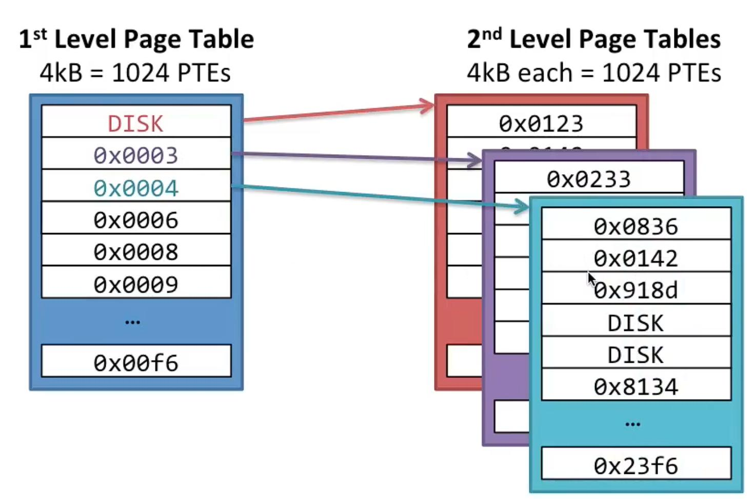
A first-level page table indexes into second-level tables whose entries are physical addresses (or DISK). The KV-cache analogue: a request’s logical block index maps, through the page table, to whatever physical KV page the allocator had free — the mapping, not adjacency, defines the layout.
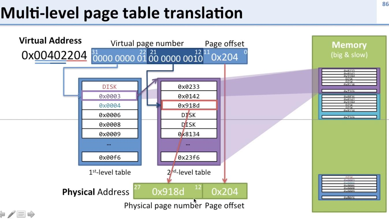
The same idea end to end: a logical/virtual address is split into page-table indices plus an offset; translation walks the tables to a physical page number, and the offset is contiguous within that page. FlashInfer keeps exactly this shape — scatter at page granularity, contiguous within a page (the head dimension).
Now the move Figure 2 makes: that page table can be interpreted as a sparse matrix whose rows are query tiles and columns are physical KV pages. [Paper]
             Physical KV pages
             P0 P1 P2 P3 P4 P5 ...
           ┌────────────────────────
Request 1  │  ✓  ✗  ✓  ✗  ✗  ✓         →  [ 1 0 1 0 0 1 ]
Request 2  │  ✗  ✓  ✓  ✗  ✓  ✗
Request 3  │  ✓  ✗  ✗  ✓  ✗  ✗
           └────────────────────────
                Block Sparse Matrix
One rule reads the whole figure: a non-zero block means “this query tile accesses this physical KV page.” The 1s mean access these; the 0s are an absence of work, not stored zeros. The two block-size parameters: [Paper]
| Symbol | Meaning | Who chooses it |
|---|---|---|
| $B_r$ | Query tile size — queries grouped into one row block | FlashInfer / kernel config |
| $B_c$ | KV block (page) size | The KV-cache management algorithm (serving system) |
Figure 2 uses $B_r=4$, $B_c=1$. And crucially, FlashInfer supports arbitrary $(B_r,B_c)$ — because $B_c$ is someone else’s decision, the kernel cannot dictate the page size and must handle whatever the memory manager picked. That is exactly the arbitrary-$B_c$ point from §IV.2, now with a name for the parameter. [Paper]
One more thing Figure 2 shows: the Q/O tensors are ragged (jagged), stored without padding, so requests with 8, 4, 4 query tokens pack compactly into one tensor. K/V start as ragged tensors too (sharing Q’s index pointers, since all come from $W_q,W_k,W_v$ on the same input) and only afterwards get incorporated into the KV cache. [Paper] So:
| Tensor | Format | Why |
|---|---|---|
| Q / O | Ragged (row-offset indexed) | Variable query lengths, packed with no waste |
| KV cache | BSR (block-sparse) | Variable, non-contiguous physical placement |
IV.5 This is not sparse GEMM — the misreading to avoid
The tempting reading is “$QK^\top$ where $K$ is sparse, so do a sparse matrix multiply.” Wrong. The BSR structure supplies an access pattern; the computation over the selected data stays dense. Nothing is copied or rearranged either — given L0→P7, L1→P2, L2→P15, FlashInfer keeps the KV cache where it is and consults the mapping. Confirmed in §3.2.1: the composable-format approach “doesn’t require data movement in the KV cache; instead, we compute the indices and index pointer arrays for the sparse submatrices.” [Paper]
The page table telling me where my KV blocks live can itself be represented as a BSR structure. The attention kernel then uses that structure to decide which physical KV blocks each query tile should access. [Interpretation]
IV.6 Composable formats (Figure 3): the second reason ⊕ exists
A single BSR format is stuck with a fixed block size, and $B_r$ is doing double duty: [Paper]
| Larger $B_r$ | Smaller $B_r$ |
|---|---|
| ✅ Better shared-memory/register reuse for requests within the same block | ✅ Less fragmentation |
| ❌ More fragmentation | ❌ No cross-query reuse |
The insight that made Figure 3 click for me: $B_r$ is really a memory-tier selector. Queries in the same block are in the same threadblock, and a threadblock owns a shared-memory allocation — so $B_r$ decides which level of the hierarchy serves the KV data. [Interpretation]
        Throughput ▲
            │       ┌──────┐
            │       │ Reg  │
            │      ┌┴──────┴┐
            │      │  SMEM  │   ◄── B_r = 3: three queries share one KV tile here
            │     ┌┴────────┴┐
            │     │ L2 Cache │
            │    ┌┴──────────┴┐
            │    │   Global   │  ◄── B_r = 1: each query fetches its own KV, from here
            └────┴────────────┴──►
So B_r = 3 vs B_r = 1 is the difference between reading a KV tile once from SMEM for three queries and reading it three times from global memory. Rather than picking one $B_r$ and living with the trade-off, composable formats use several BSR matrices, each with the block size suited to its structure. Shared prefixes are the obvious case: if requests share a prefix, the corresponding rows/columns form a dense submatrix, which a large $B_r$ is good at. [Paper]
Full KV-cache sparse matrix
            │  decompose on known structure
            ▼
  ┌─────────────────────┬──────────────────────┐
  │  shared prefix      │  unique suffix        │
  │  (dense submatrix)  │  (genuinely sparse)   │
  │  BSR, B_r = 3       │  BSR, B_r = 1         │
  │  → SMEM / registers │  → global / L2        │
  └─────────────────────┴──────────────────────┘
Two corrections again: nothing is grouped or copied — the paper is explicit that it “doesn’t require data movement in the KV cache; instead, we compute the indices and index pointer arrays.” Two views are constructed over the same physical bytes. And FlashInfer never inspects tokens — the serving system’s radix tree/page table already knows which requests share a prefix; FlashInfer just turns that relationship into BSR indices a kernel can exploit. [Paper]
Now the part I hadn’t anticipated: this is why ⊕ exists. The two block-sparse matrices produce separate attention states that must be combined:
 Block size (1,1)          Block size (3,1)
 unique KV-Cache            shared KV-Cache
        │                          │
        ▼                          ▼
   [O₁, lse₁]        ⊕        [O₂, lse₂]
        └─────────────┬────────────┘
                      ▼
              [O_all, lse_all]
So decomposing the format forces a recombination step, and the operator is exactly §III’s ⊕. This reframes ⊕ for me — I had filed it under “load balancing.” It has two independent motivations, one operator: [Interpretation]
| Use of ⊕ | What’s being split | Why |
|---|---|---|
| §3.3 scheduler | One KV sequence → chunks across CTAs | Load balance / SM occupancy |
| §3.1.2 composable formats | One KV matrix → submatrices by block size | Memory-tier optimisation |
That is why the paper’s first contribution reads “block-sparse and composable formats” as one item, and why ⊕ had to be established in the background rather than alongside the scheduler: composability is a property of the format, and ⊕ is what makes the format decomposable at all.
IV.7 The division of labour that keeps recurring
PageAttention/RadixAttention/tree-attention are producers of a layout, not prerequisites of the engine. The paper lists page tables, radix trees, tree attention (speculative decoding), and importance masks as patterns BSR can represent; separately, it lists vLLM/SGLang/MLC-Engine as integration targets — it never joins the two into a one-pattern-per-system table, and I shouldn’t either. [Paper] The accurate statement, weaker and more correct than “FlashInfer replaces the KV-cache manager”:
FlashInfer provides a common block-sparse representation for different KV-cache storage/access patterns, allowing the same attention engine to handle them efficiently. The serving system chooses the policy (allocation, eviction, reuse); FlashInfer executes the consequence. [Interpretation]
V. From BSR to a CUDA Kernel: Indexing, Gather, and Shared Memory
Section IV is the abstraction; this section is where col_indices[idx] becomes a physical address and scattered pages become a dense tile in shared memory. I’ll build it in the order I actually understood it: a deliberately tiny kernel that isolates the one idea (BSR indexing), then the exact list of what a real kernel adds, then the paper’s real data path (§3.2.1).
V.1 Expressing Figure 2’s BSR rows as index arrays
Setup: H=1 head, D=4 head dim, B_c=1 token per page, B_r=4 queries per tile. Request 1’s logical KV maps to scattered physical pages L0→P3, L1→P5, L2→P1 — logical order L0→L1→L2, physical order P3→P5→P1. That’s the non-contiguity. With two query tiles, the occupancy matrix becomes two flat arrays — the entire page table: [Educational]
// BSR row pointers: tile i owns col_indices[row_ptr[i] .. row_ptr[i+1])
int row_ptr[]     = { 0, 3, 5 };          // tile 0 → [0,3), tile 1 → [3,5)
// Physical KV page ids for each non-zero BSR block.
int col_indices[] = { 3, 5, 1,   2, 4 };  // tile 0 → P3,P5,P1 ; tile 1 → P2,P4
row_ptr says how many pages a tile touches; col_indices says which ones.
V.2 The toy kernel
Not FlashInfer’s actual kernel — the point is to isolate BSR indexing, then map every gap to a real feature. [Educational]
#include <cuda_runtime.h>
#include <cmath>

// Br = queries per tile, D = head dimension. Both are template parameters (not runtime
// args) because output[D] is a register array, and register arrays need a compile-time bound.
template <int Br, int D>
__global__ void block_sparse_attention(
    const float* __restrict__ Q,            // [num_queries, D]
    const float* __restrict__ K_cache,      // [num_pages,   D]
    const float* __restrict__ V_cache,      // [num_pages,   D]
    const int*   __restrict__ row_ptr,      // [num_query_tiles + 1]
    const int*   __restrict__ col_indices,  // physical KV page ids
    float*       __restrict__ O,            // [num_queries, D]
    int num_query_tiles)
{
    const int tile_id = blockIdx.x;
    if (tile_id >= num_query_tiles) return;

    const int query_start = tile_id * Br;
    const int start = row_ptr[tile_id];        // this tile's BSR row: the slice of
    const int end   = row_ptr[tile_id + 1];    // col_indices it owns

    for (int q_local = 0; q_local < Br; ++q_local) {
        const int    q_id = query_start + q_local;
        const float* q    = &Q[q_id * D];

        float output[D];
        for (int d = 0; d < D; ++d) output[d] = 0.0f;
        float denominator = 0.0f;

        // Iterate ONLY over the non-zero BSR blocks.
        for (int idx = start; idx < end; ++idx) {
            const int physical_page = col_indices[idx];   // ← BSR becomes a physical address
            const float* K = &K_cache[physical_page * D];
            const float* V = &V_cache[physical_page * D];

            float score = 0.0f;                            // ---- Q · K ----
            for (int d = 0; d < D; ++d) score += q[d] * K[d];
            score /= sqrtf(static_cast<float>(D));

            const float weight = expf(score);              // ---- softmax (naive; see V.3) ----
            denominator += weight;

            for (int d = 0; d < D; ++d) output[d] += weight * V[d];   // ---- weight * V ----
        }
        for (int d = 0; d < D; ++d) O[q_id * D + d] = output[d] / denominator;  // normalize
    }
}
// Launch: one block per query tile → block_sparse_attention<4,4><<<num_query_tiles, 1>>>(...);
The one line that matters is const int physical_page = col_indices[idx]; — the abstract BSR structure becoming a concrete KV-cache address. The kernel is completely indifferent to the pages being non-adjacent; it follows the mapping. And the zeros were never represented — the loop bound is the sparsity: for (idx = start; idx < end; ++idx) runs 3 iterations, not 6, and never issues a load for the absent pages. That is concretely what “skip empty blocks, reducing computational overhead” means.
V.3 What the toy gets wrong — the map to a real kernel
Each gap is a real FlashInfer feature: [Interpretation]
| Gap in the toy | What a real kernel does |
|---|---|
One thread per block — threadIdx never used |
Warps cooperate; threads split the $D$ loop and the page loop |
Unsafe softmax — expf(score) overflows |
Online softmax with a running max (§II.2 recurrence) |
| No shared memory — each of $B_r$ queries re-reads the same page from global | Gather the page into shared memory once, reuse across all $B_r$ queries |
| Scalar FMA loops for $Q\cdot K$ and weight·$V$ | Tensor Core mma on tiles |
| One CTA owns the whole BSR row | Split long rows across CTAs, emit $[O,\mathrm{LSE}]$, contract with ⊕ (§VIII) |
That third row is the important one: re-reading a page $B_r$ times throws away exactly the reuse BSR was chosen to enable — the memory-tier point from §IV.6, now visible as a concrete kernel defect.
V.4 The real data path (§3.2.1): gather scattered global → contiguous shared
Stripped of jargon, §3.2.1 answers one question: if my KV cache is scattered around GPU memory, how do I efficiently get the pieces I need into the fast memory where Tensor Cores can compute? The contradiction: the computation wants dense tiles, the storage is scattered, and the pages one query needs are not adjacent. [Interpretation]
First, the memory vocabulary, because “global → shared” is meaningless without it: global memory ≈ HBM (large, slow, all SMs see it — the KV cache lives here), and shared memory belongs to an SM (not one giant pool). A block on SM0 uses SM0’s SMEM. This is exactly the hardware fact that made Figure 3 work — “requests in different blocks cannot access each other’s shared memory” isn’t a software rule, it’s this partition. [Explanatory CUDA]
Why can’t Tensor Cores just read the scattered pages? Because MMA instructions operate on fixed matrix tile shapes, and the paper states the constraint precisely: [Paper]
Tensor core inputs for a single MMA instruction can originate from different blocks within a block-sparse matrix.
So the gather isn’t an optimisation, it’s a correctness enabler: one instruction’s operand spans blocks that aren’t neighbours. The end-to-end flow:
flowchart LR
    BSR["<b>BSR indices</b><br/>'I need pages 7, 2, 19, 4'"] --> K["CUDA kernel<br/>computes addresses"]
    K -->|"scattered reads"| G["Global memory / HBM"]
    G -->|"async copy (LDGSTS)"| S["<b>Shared memory</b><br/>contiguous tile"]
    S --> TC["Tensor Cores"]
    TC --> O["Q × Kᵀ → softmax → × V"]
    style S fill:#dbeafe,stroke:#2563eb,stroke-width:3px
    style BSR fill:#fef3c7,stroke:#d97706
The paper is specific about the mechanics. Sparse KV addresses come from the BSR indices arrays; dense ones use row-index affine transformations — same kernel, different address arithmetic. That is the only difference between the two halves of Figure 4: [Paper]
| KV cache is… | Address computation | Meaning |
|---|---|---|
| Sparse / non-contiguous | page = indices[i] |
explicit mapping — a lookup |
| Dense / contiguous | address = base + row * stride |
affine — no page table needed |
Here is the gather-into-shared-memory + online-softmax structure the toy kernel was missing, written as a representative sketch — the sparse/dense split is a compile-time template parameter (see §VII), and the head-dimension load is 128-byte-wide and asynchronous: [Educational]
// Representative decode microkernel: gather scattered KV pages into shared memory ONCE,
// then run online-softmax attention over the contiguous tile. IS_SPARSE picks the
// address arithmetic at compile time — "variations only in data loading modules".
template <int Br, int D, bool IS_SPARSE>
__global__ void attention_gather(
    const float* __restrict__ Q, const float* __restrict__ K_cache,
    const float* __restrict__ V_cache, const int* __restrict__ row_ptr,
    const int* __restrict__ col_indices, float* __restrict__ O, int num_tiles)
{
    extern __shared__ float smem[];        // [tile_kv * D] staging for one KV tile
    float* K_sh = smem;

    const int tile = blockIdx.x;
    const int start = row_ptr[tile], end = row_ptr[tile + 1];

    float m = -INFINITY, l = 0.0f;          // running max, running denominator (the LSE encoding)
    float acc[D];
    #pragma unroll
    for (int d = 0; d < D; ++d) acc[d] = 0.0f;

    for (int idx = start; idx < end; ++idx) {
        // --- data-loading module: the ONLY part that differs sparse vs dense ---
        int page;
        if constexpr (IS_SPARSE) page = col_indices[idx];        // lookup
        else                     page = idx;                     // affine: base + row*stride
        const float* K_src = &K_cache[page * D];

        // Coalesced, 128B-wide async copy of the head vector into shared memory.
        // Threads of the warp cooperate; the last dim (D) is contiguous, so this is one wide txn.
        for (int d = threadIdx.x; d < D; d += blockDim.x)
            K_sh[d] = K_src[d];              // stand-in for cp.async / LDGSTS
        __syncthreads();

        // --- from here down, sparse and dense CONVERGE: identical FlashAttention math ---
        float score = 0.0f;
        for (int d = 0; d < D; ++d) score += Q[d] * K_sh[d];
        score *= rsqrtf((float)D);

        const float m_new = fmaxf(m, score);           // online-softmax update (§II.2)
        const float corr  = __expf(m - m_new);
        const float w     = __expf(score - m_new);
        l = l * corr + w;
        const float* V_src = &V_cache[page * D];
        #pragma unroll
        for (int d = 0; d < D; ++d) acc[d] = acc[d] * corr + w * V_src[d];
        m = m_new;
        __syncthreads();
    }
    #pragma unroll
    for (int d = 0; d < D; ++d) O[d] = acc[d] / l;      // deferred normalisation
}
The paper gives the concrete data-movement facts this sketch stands in for: [Paper]
- Tiles move from scattered global memory into contiguous shared memory using
LDGSTS(load-global-store-shared, async, no register round-trip) at 128 B width to maximize bandwidth. - The last dimension of the KV cache stays contiguous (head dimension $d$, commonly 128 or 256), preserving coalesced access that fits cache lines. So the scatter is at page granularity while each page is internally contiguous — which is why
&K_cache[page * D]is a sensible access shape, not a pathological one. - Hopper’s TMA is used only for contiguous KV cache, since it doesn’t support non-affine access; sparse cases fall back to Ampere-style async copies.
Notice the pattern: the same distinction — affine vs indexed — determines the address math, the copy instruction (LDGSTS vs TMA), and the hardware unit. One property, three consequences. And the payoff line that justifies the entire BSR bet: [Paper]
Post-transfer to shared memory, the sparse and dense FlashAttention implementations converge, allowing consistent kernel usage with variations only in data loading modules.
The abstraction boundary is the shared-memory load. Above it, layout diversity — page tables, radix trees, tree attention, importance masks. Below it, one FlashAttention kernel. All the flexibility lives in how the KV address is computed; none of it leaks into the math.
VI. The Microkernel and Tile Selection (§3.2.2)
One sentence: FlashInfer does not use one fixed-size chunk of Q/K/V for every workload. It chooses a tile size that fits the particular workload and GPU. [Paper]
VI.1 Why not always (128, 64)?
Traditional FA2 uses a limited set of tile sizes (e.g. (128, 64) — 128 query rows × 64 KV positions), optimal for prefill but inefficient for shorter-query-length decoding, and one architecture’s ideal tile may not suit another (Ada/sm89 has limited shared memory, hurting occupancy with large tiles). [Paper] Two independent reasons — workload and hardware. Prefill has query ≈ KV ≈ 1024: a large tile pays off because loaded data gets reused many times. Decode has query length 1 and KV maybe 10,000:
you have:            1 query
tile is built for:   128 queries
                     ────────────
                     127/128 wasted
This is the operational-intensity result from §II showing up as a concrete tile-shape decision. Decode is $O(1)$ intensity; a prefill-shaped tile assumes it isn’t. So FlashInfer supports many tile sizes: [Paper]
\[(1, 16, 32, 64, 128) \times (32, 64, 128)\]Query tile sizes × KV tile sizes — 15 combinations, selected by heuristics on hardware resources and workload intensity. The odd gap (1, then jumping to 16) is not a coincidence: query tile size 1 uses a CUDA Cores template because the tensor-core mma minimum row count is 16 (§VII). Below 16 there are no Tensor Cores to use.
VI.2 The two heuristic steps
Step 1 — look at the batch. Determine average query length per batch, choose the minimal query tile size meeting or exceeding it. For queries 1,2,1,4 the average is 2, so the minimal size ≥ 2 from {1,16,32,64,128} is 16, not 128. [Paper] A wrinkle I’d have missed: for GQA the query length is fused with the head-group dimension, so the effective query length is $l_{qo}\times g$. A decode step with $l_{qo}=1$, $g=8$ has effective query length 8, not 1 — the same $O(g\cdot l_{qo})$ trick from §II reappearing as a tile-selection input. GQA doesn’t just improve the roofline; it changes which microkernel gets picked. [Paper]
Step 2 — fit the hardware. Formulate register and shared-memory constraints as functions of K/V tile size, maximizing SM occupancy. A small tile leaves room for many resident CTAs (good latency hiding); a large tile means one resident CTA (nothing to hide stalls behind) but more data reuse. [Paper]
          TILE SIZE
       ┌──────┴──────┐
   Smaller        Larger
       ▼             ▼
 Less memory     More memory
 Less reuse      More data reuse
 More CTAs       Fewer CTAs
 (occupancy)     (arithmetic efficiency)
This is the third appearance of the same reuse-vs-capacity tension: $B_r$ in Figure 3 (reuse vs fragmentation), tile size here (reuse vs occupancy). Same physics, different knob. [Interpretation]
VI.3 The connection to keep: $B_r = T_q$
Tile size and BSR block size are not the same thing, but the paper deliberately aligns them: the block row size $B_r$ is aligned with the query tile size $T_q$. [Paper] So choosing $T_q=16$ lets the BSR representation use $B_r=16$. This closes a loop from §IV: $B_r$ “comes from the query tile size,” and now I know what sets $T_q$ — the §VI.2 heuristics from workload and hardware. The compute side picks $B_r$; the serving system picks $B_c$. The layout parameter isn’t free-floating — half of it is a scheduling/compile decision. And critically, tile sizes resolve at compile time, so the specialization is baked into which kernel gets generated, not a runtime if (arch==sm90a) branch. That is the bridge to the JIT compiler. [Paper]
VII. The JIT Compiler and Customizable Functors (§3.2.3)
§3.2.1 handled where the data is, §3.2.2 handled how big the tile is. This subsection handles what the attention rule is — and it’s where “customizable attention engine” stops being a slogan. The mechanism: one CUDA template with holes, and a JIT compiler that fills the holes with user-supplied code.
VII.1 The template with holes
The skeleton never changes; the bracketed pieces do:
              CUDA TEMPLATE
       ┌─────────────────────────┐
       │ Load Q                  │  ← §3.2.1 machinery
       │ Load K                  │
       │ Load V                  │
       │                         │
       │ [CUSTOM Q TRANSFORM]    │
       │                         │
       │ Q × K                   │  ← §3.2.2 tile machinery
       │                         │
       │ [CUSTOM LOGITS]         │
       │ [CUSTOM MASK]           │
       │                         │
       │ Softmax  (optional!)    │
       │                         │
       │ × V                     │
       │                         │
       │ [CUSTOM OUTPUT]         │
       └─────────────────────────┘
The paper calls the bracketed pieces functors, and pins the contract precisely: [Paper]
Each functor has a fixed signature that takes the kernel parameters, input and current query/key/head index as input, and returns the output. Those variant functions are specified as member of a user-defined variant class which creates a closure for the variant functors.
The fixed signature is what makes it work: the template can call a hole without knowing what fills it, and the closure carries per-variant state (scale, bias, window size) alongside. A functor here is just a small piece of CUDA/C++ logic that performs one customizable operation inside the attention kernel.
VII.2 The six customization points
| Functor | Where it acts | Example use |
|---|---|---|
QueryTransform |
Q, before attention | RoPE, normalization, projection |
KeyTransform |
K, before attention | RoPE, normalization, projection |
ValueTransform |
V, before attention | — |
LogitsTransform |
on $S = QK^\top$, before softmax | logits soft-cap, sigmoid |
LogitsMask |
on $S$, before softmax | causal, sliding window, custom masks |
OutputTransform |
on $O$, before returning | post-scaling etc. |
Three of these earn a specific paper-credited win: [Paper]
- Q/K/V transforms → fusion. The query/key transformation functors make it possible to fuse normalization, RoPE, and projection into the attention kernel — eliminating separate kernel launches and HBM round-trips for what would otherwise be their own passes.
- LogitsMask → masks as computation, not memory. Causal, sliding-window, and custom masks become a predicate evaluated in-register (
can attend? no → S[i,j] = -∞). For long context this is the difference between an $O(l^2)$ mask tensor and no tensor at all. -
Softmax is optional. The one I didn’t expect: [Paper]
FlashInfer has an option of using softmax or not in the attention variant specification, which makes it capable of supporting attention variants that don’t use softmax, such as FlashSigmoid.
So “attention engine” is scoped more broadly than “softmax attention engine” — the online-softmax machinery from FA2 (§II) is itself behind a switch.
LogitsTransformandLogitsMaskare the two the paper credits directly to FlexAttention, the intellectual debt for this subsection.
VII.3 How the JIT part runs
Ask for FlashSigmoid and the specification says, in effect: LogitsTransform = scale, bias, sigmoid; Softmax = NO. Then:
flowchart TD
    S["<b>Attention specification</b><br/>(Python, containing CUDA source strings)"]
    S --> J["<b>JIT compiler</b><br/>insert variant class + info into template"]
    J --> G["Generated CUDA source"]
    G --> C["Compiled with <b>PyTorch's JIT compiler</b>"]
    C --> R["Registered as a <b>custom operator</b>"]
    R --> K["GPU kernel, callable from the serving system"]
    C -.->|"framework-agnostic path"| D["<b>DLPack</b> → other runtimes"]

    style J fill:#dbeafe,stroke:#2563eb,stroke-width:3px
    style S fill:#fef3c7,stroke:#d97706
Which is what puts the “Just-In-Time” in JIT: the kernel doesn’t exist until the variant is known. Two details that matter more than they look: [Paper]
- The spec accepts raw CUDA code to define the functors, which “enables user to use advanced PTX instructions or even their own libraries.” The extension point isn’t a fixed menu — it’s an arbitrary code-injection site. Much stronger than “configurable.”
- Compilation to other runtime systems is supported through the framework-agnostic DLPack interface, so PyTorch isn’t the only path.
VII.4 Reading Figure 5: FlashSigmoid concretely
Figure 5 maps FlashSigmoid across five panels — the Python spec on the left, and the four places its pieces land in generated CUDA: kernel parameters class, kernel traits class, kernel body, PyTorch custom-op registration. The variant class (abridged from the figure): [Paper]
template <typename Params_, typename KernelTraits_>
struct FlashSigmoid {
    using Params       = Params_;
    using KernelTraits = KernelTraits_;

    static constexpr bool use_softmax = false;   // ← the softmax switch

    float scale, bias;

    __device__ FlashSigmoid(const Params& params, int batch_idx, uint8_t* smem_ptr) {
        // Copy from CUDA constant memory to registers
        scale = params.scale;
        bias  = params.bias;
    }

    __device__ float LogitsTransform(const Params& params,
                                     float logit_score,
                                     int b_idx, int q_idx, int kv_idx,
                                     int qo_head_idx, int kv_head_idx) {
        return 1.f / (1.f + expf(-(logit_score * scale + bias)));
    }
};
So instead of logits → softmax, FlashSigmoid does logits → scale × logits + bias → sigmoid. The constructor is where “creates a closure” becomes concrete: scale and bias are pulled from constant memory into registers once, then reused by every LogitsTransform call. The kernel body invokes it per element of the in-register logits tile:
// Iterate over all elements inside the thread logits tile
for (int i = 0; i < num_elements; ++i) {
    auto [qo_idx, kv_idx] = get<i>(logits_tile);     // register index → (q, kv)
    logits_tile(i) = attn.LogitsTransform(params, logits_tile(i),
                                          batch_idx, qo_idx, kv_idx,
                                          qo_head_idx, kv_head_idx);
}
Note where: on logits_tile, already in registers. The transform never touches HBM — that’s why fusing a variant here is nearly free, and why the functor needs the index arguments (it must reconstruct which $(q, kv)$ pair a register slot maps to). The traits class carries the compile-time facts:
struct KernelTraits : AttentionSpec {
    static constexpr HEAD_DIM  = ;
    static constexpr IS_SPARSE = ;
};
IS_SPARSE is the sighting that closes §V: the sparse/dense split is a constexpr template parameter, not a runtime branch. “Variations only in data loading modules” is literally a compile-time constant. Then the whole thing is instantiated and registered as a Torch custom op:
auto kernel = KernelTemplate<FlashSigmoid<Params, KernelTraits>>;
TORCH_LIBRARY_IMPL("FlashSigmoid", CUDA, m) {
    m.impl("run", &attention_custom);
}
Same skeleton, different attention rule.
VII.5 Why generation instead of hand-writing
The specialization axes multiply: attention variants × 15 tile combinations × head dimensions × GPU architecture (FA2/FA3) × dense/sparse. Writing that product by hand is hopeless; generating it is routine. The JIT compiler is not a convenience feature — it’s the only tractable way to cover the cross-product that §VI and §V create. [Interpretation]
VIII. The Dynamic Load-Balanced Scheduler (§3.3)
The previous three subsections built a fast, customizable kernel. This one asks the serving question: given a batch where one request has 30 tokens of KV and another has 30,000, and where those lengths change every generated token, how do you keep every SM busy — without breaking CUDAGraph? The paper’s own framing of the constraint pair: [Paper]
FlashInfer employs a dynamic load-balanced scheduling framework to handle input dynamism … while maintaining compatibility with CUDAGraph’s requirement for constant configurations.
Two forces pulling opposite ways:
dynamism wants:      a different launch every step (lengths changed)
CUDAGraph wants:     the exact same launch every step (that's the whole point)
CUDAGraph captures a fixed graph of kernel launches to kill per-launch CPU overhead — so the launch configuration cannot change per step. The scheduler’s job is to absorb all the dynamism without touching the launch.
VIII.1 Why chunking is what makes balancing possible
Four requests of wildly different KV lengths are four lumpy work units — hand them to four CTAs and the long one runs while three sit idle. Chunking (legal only because ⊕ is associative — §III) splits each request’s KV into bounded pieces, so the scheduler holds many small units instead of a few lumpy ones. This is the second, independent use of ⊕: not merging paged KV for one query (§IV), but splitting one long sequence for load balance. Same operator, different motive. [Interpretation]
VIII.2 Algorithm 1 = LPT greedy
The cost model, with $\alpha,\beta$ hyperparameters, and the max KV chunk size given query tile $T_q$ and CTA count: [Paper]
\[\mathrm{cost}(l_q, l_{kv}) = \alpha \, l_q + \beta \, l_{kv} \qquad L_{kv} \leftarrow \frac{\sum_i \left\lceil \dfrac{l_{qo}(i)}{T_q} \right\rceil \cdot l_{kv}(i)}{\#\mathrm{CTA}}\]That numerator is total work across the batch; dividing by #CTA gives the ideal per-CTA share — so the chunk size is derived from “what would perfect balance look like,” not picked arbitrarily. Then the assignment loop:
- Split each query tile’s KV into chunks of at most $L_{kv}$; each chunk is a work item.
- Sort all work items descending by length.
- Put the CTAs in a min-priority-queue keyed by accumulated cost.
- Repeatedly: pop the least-loaded CTA, pop the largest remaining work item, assign it, push the CTA back with updated cost.
sort work descending  +  always give it to the emptiest CTA
        = Longest-Processing-Time-first greedy (LPT)
The standard greedy approximation for multiprocessor scheduling; the paper credits Stream-K (Osama et al., 2023) as inspiration. As a representative CPU-side sketch of the plan step: [Educational]
// Runs on the CPU, once per generation step. Produces the plan the GPU kernels read.
struct WorkItem { int req_id, kv_start, kv_len; };     // one KV chunk
struct CTA      { float cost; int id; };
struct CTACmp   { bool operator()(const CTA& a, const CTA& b) const { return a.cost > b.cost; } };

std::vector<std::vector<WorkItem>> plan_lpt(
    const std::vector<int>& l_qo, const std::vector<int>& l_kv,
    int Tq, int num_ctas, float alpha, float beta)
{
    // L_kv = total work / #CTA  → the ideal per-CTA share
    long total = 0;
    for (size_t i = 0; i < l_kv.size(); ++i)
        total += (long)std::ceil((double)l_qo[i] / Tq) * l_kv[i];
    const int L_kv = std::max(1L, total / num_ctas);

    // 1. chunk every request's KV into pieces of at most L_kv
    std::vector<WorkItem> work;
    for (size_t r = 0; r < l_kv.size(); ++r)
        for (int s = 0; s < l_kv[r]; s += L_kv)
            work.push_back({(int)r, s, std::min(L_kv, l_kv[r] - s)});

    // 2. sort work items DESCENDING by length (the "Longest-Processing-Time-first")
    std::sort(work.begin(), work.end(),
              [](const WorkItem& a, const WorkItem& b){ return a.kv_len > b.kv_len; });

    // 3. min-heap of CTAs keyed by accumulated cost
    std::priority_queue<CTA, std::vector<CTA>, CTACmp> heap;
    for (int c = 0; c < num_ctas; ++c) heap.push({0.f, c});

    // 4. always hand the next-largest item to the emptiest CTA — DETERMINISTIC given same lengths
    std::vector<std::vector<WorkItem>> queues(num_ctas);
    for (const auto& w : work) {
        CTA least = heap.top(); heap.pop();
        queues[least.id].push_back(w);
        least.cost += alpha * l_qo[w.req_id] + beta * w.kv_len;   // cost(l_q, l_kv)
        heap.push(least);
    }
    return queues;   // work queue per CTA — half the plan; the other half is the reduction map
}
VIII.3 Determinism: no atomics
The paper deviates from Stream-K deliberately: [Paper]
because LLM serving requires deterministic outputs, we did not incorporate atomic aggregation … The scheduling algorithm generates deterministic aggregation order when provided with identical sequence length information.
Atomics would be the obvious way to reduce partials, but floating-point addition isn’t associative in finite precision, so a race-determined order gives run-to-run variation in the output logits. FlashInfer pins the aggregation order in the plan: same lengths in → same reduction order → bitwise-reproducible out. Note the exact tension: ⊕ is mathematically associative (which makes partitioning legal), but only approximately so in floating point (which is why the schedule fixes one order). Free to partition, not free to reorder at runtime.
VIII.4 CPU plans, GPU computes
The natural fear — partial states shipped to the CPU for reduction, catastrophic for latency — is not what happens:
flowchart TD
    subgraph CPU
        SL["sequence length info<br/>(query/output + key/value dims)"] --> SCHED["Runtime Scheduler<br/>(Algorithm 1 / LPT)"]
        SCHED --> PLAN["<b>Plan information</b><br/>1. work queue per CTA<br/>2. partial→final index map"]
    end
    PLAN -->|"async copy to fixed<br/>workspace offset"| WS["<b>GPU Workspace Buffer</b><br/>plan info + partial outputs"]
    subgraph GPU
        WS --> AK["Attention Kernel<br/>(persistent)"]
        AK --> PS["partial attention states<br/>[Oᵢ, LSEᵢ]"]
        PS --> CK["Contraction Kernel (persistent)<br/>⊕ over partials"]
        CK --> OUT["Final attention output"]
    end
    style CPU fill:#fef3c7,stroke:#d97706
    style GPU fill:#dbeafe,stroke:#2563eb
    style PLAN fill:#fde68a,stroke:#d97706
The CPU computes the plan and async-copies it to a fixed region of the GPU workspace. It never computes $QK^\top$, never computes $\mathrm{softmax}(QK^\top)V$, never performs the reduction — its entire contribution is “here is the work schedule.” And the paper inverts the naive expectation about the attention kernel’s output: [Paper]
The attention kernel does not produce the final output directly because some long KV are split into multiple chunks, and the final output is the contraction … of all chunks’ partial outputs.
So the attention kernel’s declared output is a partial state $[O_i, \mathrm{LSE}_i]$; producing final answers is a separate stage’s job.
VIII.5 The reduction map (Figure 6)
The scheduler emits two things: a work queue per CTA, and an index mapping between partial and final outputs — the reduction map. Figure 6’s shape: [Paper]
final 0 ← partial [8]          final 3 ← partial [4]
final 1 ← partial [1, 2]       final 4 ← partial [5, 6]
final 2 ← partial [3]
The structural point: some final outputs come from a single partial, others from several. A short request was never split, so its partial is its answer; a long request was split, so its answer is a ⊕-contraction. The map is what lets one uniform kernel handle both — variable-length aggregation.
VIII.6 Plan reuse and CUDAGraph compatibility
The scheduler runs per generation step, but a 32-layer model doesn’t need 32 planning passes — every layer in a step attends over the same sequence lengths, so the plan is computed once and reused across all layers, amortizing the cost. [Paper] And the CUDAGraph loop finally closes:
| Requirement | How it’s met |
|---|---|
| Constant grid size | Attention + contraction use persistent kernels; grid fixed at compile time |
| Constant kernel arguments | Fixed offsets in the workspace buffer — the pointers never change |
| Varying workload | Dynamism lives in the workspace contents (the plan), not the launch config |
FlashInfer even merges attention and contraction into one persistent kernel to eliminate intra-kernel overhead. And the plan/run split (the Inspector-Executor model): plan runs on the CPU and is not captured by CUDAGraph; run is the captured graph, replayed each step reading the new plan from the workspace. [Paper]
per generation step:
    plan(seqlen_info)     ← CPU, not captured
    graph.replay()        ← GPU, fixed launch, reads the new plan from workspace
The synchronisation point (a final output waits on all its partials) doesn’t vanish — FlashInfer makes it cheap rather than absent: chunk, distribute via LPT, emit partials, contract on-GPU with persistent fixed-grid kernels. Continuous batching governs requests entering/leaving the workload; the scheduler governs keeping the SMs saturated within a step. Different levels, not the same job.
IX. Figure 1: The Whole System on One Page
Everything above is one box in Figure 1 (page 2), the paper’s system-design overview. It’s drawn as two panels split by a dashed diagonal, and that divide is the paper’s central separation — what the workload is vs how the GPU executes it.
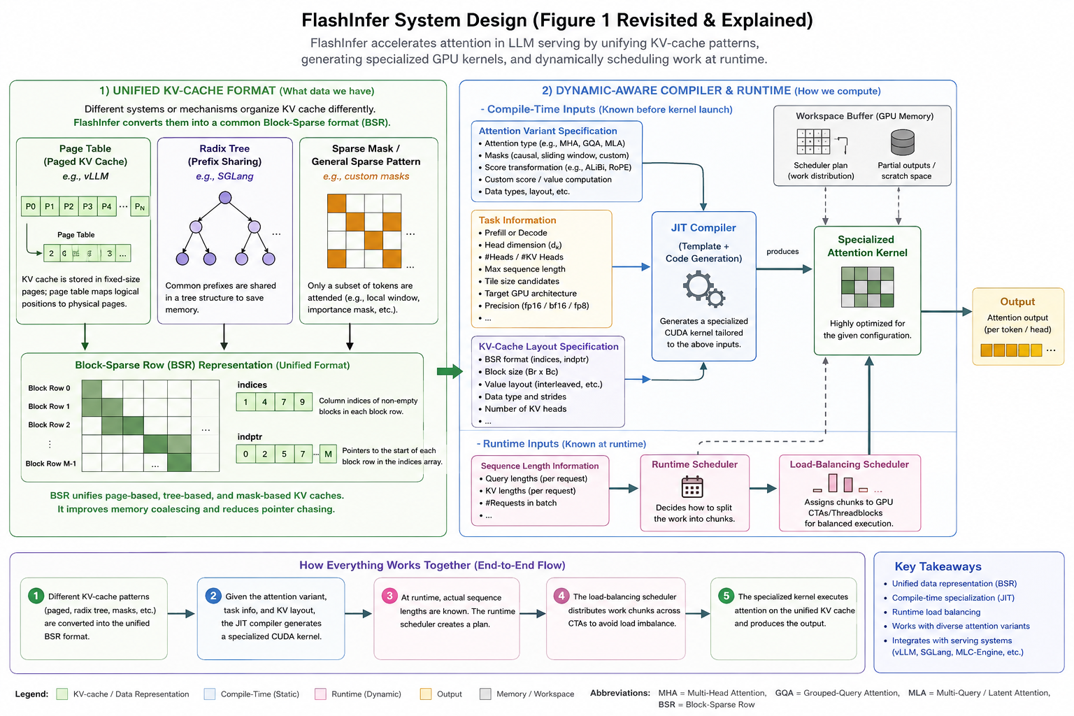
FlashInfer's design in one figure: heterogeneous KV-cache layouts (page table, radix tree, sparse mask) collapse into a single block-sparse representation on the left; a JIT compiler (compile time) and a load-balancing scheduler (run time) feed one attention kernel on the right.
IX.1 The left panel — layout diversity collapses to one representation
Three visually different KV-cache organizations — a page table, a radix tree, a sparse mask — all funnel into one data structure: a block-sparse matrix. That’s §3.1 stated pictorially: the kernel below doesn’t need to know which of the three it came from. The alternative — the thing FlashInfer refuses to do — is maintain a RadixAttention kernel and a PagedAttention kernel and a TreeAttention kernel and a SparseMask kernel, each separately optimized. One abstraction in, one kernel path out. (These are access patterns, not system name-tags — the figure isn’t labelling one per engine.) [Interpretation]
IX.2 The right panel — two feeders, fed at different times
Query and KV flow into a single Attention Kernel producing the Output — but that kernel isn’t a fixed artifact. Two boxes feed it, at different times: [Paper]
| Box | Fed by | When |
|---|---|---|
| JIT Compiler | attention-variant spec, task information, KV-cache layout spec | compile time |
| Load-balancing Scheduler | sequence length information | run time |
The paper’s caption says exactly this. The three compile-time inputs, one at a time: (1) Attention Variant Specification — what kind of attention (grouped heads, custom masks, custom score computation)? (2) Task Information — what workload (prefill/decode, head dim, query/KV length, target hardware, tile config, sparse/dense)? (3) KV-Cache Layout Specification — the box that stitches the two panels together, because layout determines the generated data-loading code (dense → affine addressing; sparse → indices/indptr → gather). [Paper]
Both the compiler and scheduler live inside the Workspace Buffer — FlashInfer’s own persistent working memory holding plan information and partial attention outputs. That persistence is exactly what keeps the launch config constant for CUDAGraph (§VIII.6).
IX.3 The split that is the real idea
known ahead of time  ──►  JIT compile it away        (variant, layout, tiles)
changes every step   ──►  schedule it at runtime     (sequence lengths → CTA work chunks)
So Figure 1 isn’t really an architecture diagram — it’s the paper’s argument in picture form: unify the layouts, generate the kernel, schedule the work. Mapped onto the four-stage chain: [Interpretation]
Left panel                    Right panel
────────────                  ─────────────────────────────────────
BSR for the KV cache    →     CUDA/CUTLASS templates + JIT compiler  →  load-balancing scheduler
   (§3.1)                              (§3.2)                               (§3.3)
   memory dimension                 compute dimension                     dynamism
X. Where FlashInfer Sits: Two Dimensions, Not Two Teams
A tempting-but-wrong summary: “TensorRT-LLM and SGLang work the memory side, FlashInfer works the hardware side.” That’s not the paper’s split. It separates two dimensions of the problem, and FlashInfer sits across both. [Interpretation]
- Dimension 1 — memory/data: how is the KV cache represented and accessed? (paged attention, radix trees, block-sparse, prefix sharing). FlashInfer owns this via BSR.
- Dimension 2 — compute/hardware: how is attention executed efficiently? (CUDA/CUTLASS templates, tile sizes, Tensor Cores, shared memory, scheduling). FlashInfer owns this via §3.2–3.3.
The paper’s claim for why it must span both: different KV-cache organizations create memory-access problems, and different GPU workloads require different kernel implementations. You can’t fix one without the other — a perfect kernel over a badly-expressed layout still does scattered global reads; a unified layout with one rigid kernel still wastes Tensor Cores. [Paper]
X.1 The deployment boundary
FlashInfer is designed to slot underneath an existing serving system, not replace it. Two mechanisms (both §3.2.3): PyTorch stacks get generated CUDA compiled with PyTorch’s JIT and registered as a custom operator; everything else uses the framework-agnostic DLPack interface. So: serving framework handles the model and request side → FlashInfer handles attention execution → CUDA runs it on the GPU. [Paper]
X.2 Isn’t this TensorRT-LLM’s in-flight batching?
Half right — in-flight batching (IFB) does attack dynamism, but at a different layer. The two questions don’t overlap: [Paper]
TensorRT-LLM IFB asks: “Which requests should I execute together in this iteration?”
FlashInfer’s scheduler asks: “Given the work I have, how do I distribute it across CTAs so no SM idles?”
IFB governs request admission (Level 1); FlashInfer’s scheduler governs CTA-level load balance within a step (Level 2). They compose — TensorRT-LLM can use FlashInfer as an attention backend in its PyTorch backend, the same relationship as SGLang and vLLM.
X.3 The full stack (my synthesis, beyond the paper’s scope)
Calibration: the FlashInfer paper’s scope stops at the serving-engine interface — it names vLLM, SGLang, MLC-Engine as integration targets and says nothing about distributed KV infrastructure. Mooncake is my own addition to place FlashInfer in its ecosystem, not something the paper claims. [Interpretation]
flowchart TD
A["LLM application · Chat / Agents / API"] --> M
subgraph MC[" MOONCAKE — distributed KV infrastructure (NOT in the paper) "]
M["KV-cache transfer & pooling · RDMA<br/><i>where is the KV cache, how do I move it?</i>"]
end
M -->|"supplies / moves KV"| SE
subgraph SE[" SERVING ENGINE — vLLM / SGLang / MLC-Engine "]
V["scheduling · batching · KV management<br/>PagedAttention / RadixAttention"]
end
V -->|"KV layout + indices, sequence lengths"| FI
subgraph FI[" FLASHINFER — attention engine "]
API["plan( ) / run( ) API"] --> B["Block-sparse + composable formats<br/>arbitrary (B_r, B_c) · no data movement"]
API --> R["Runtime scheduler<br/>seq lengths → LPT work plan → reduction map"]
B -->|indices| K["CUDA / CUTLASS templates<br/>FA2 (sm75–89) · FA3 (sm90a) · JIT variants"]
R -->|JIT + work plan| K
end
K -->|generated kernels| GPU
subgraph GPU[" NVIDIA GPU "]
H["HBM (KV cache)"] -->|LDGSTS / TMA| SM["Shared memory (per SM)"] --> TC["Tensor Cores"] --> O["Attention output"]
end
style FI fill:#dbeafe,stroke:#2563eb,stroke-width:4px
style SE fill:#fef3c7,stroke:#d97706
style MC fill:#f3e8ff,stroke:#9333ea,stroke-dasharray: 6 4
style GPU fill:#dcfce7,stroke:#16a34a
| Layer | Owns | Does not own |
|---|---|---|
| Mooncake | KV placement/movement across devices | which requests run |
| vLLM / SGLang | admission, batching, KV organisation | how attention executes |
| FlashInfer | attention execution: layout → kernel → schedule | what to cache, what to admit |
| CUDA / GPU | instruction execution | any of the above |
Five independent routes led to the same line — the scope check on Q/K/V projections, “producers not prerequisites,” “CPU plans / GPU computes,” custom-op registration, and §5.1’s shared-prefix table — all say: FlashInfer is the execution layer, and deliberately not anything above it.
XI. Evaluation: A Validation Matrix, Not a Scoreboard
The thing not to write: “they tested it on A100 and H100 and it was faster.” What §4 actually is: each experiment validates one architectural contribution. Setup: FlashInfer v0.2, A100 40GB / H100 80GB, CUDA 12.4, PyTorch 2.4.0, FP16 storage + compute. [Paper]
| § | Experiment | Mechanism it tests | Metric | Result |
|---|---|---|---|---|
| 4.1 | End-to-end serving (SGLang) | the whole system | ITL, TTFT | 29–69% lower ITL vs Triton backend |
| 4.2 | Input dynamism | §3.3 scheduler + §3.2.2 tiles | bandwidth / FLOPs util. | beats FA2+FA3; gap largest on skewed |
| 4.3 | Long-context (Streaming-LLM) | §3.2.3 JIT / fused RoPE | ITL, bandwidth util. | 28–30% lower latency, 1.6–3.7× bandwidth |
| 4.4 | Parallel generation (MLC-Engine) | §3.1.2 composable formats | speedup | 13–17% speedup |
The metric choice is itself the §II argument: bandwidth utilization for decode, FLOPs utilization for prefill — decode is $O(1)$ intensity so bandwidth is the ceiling; reporting FLOPs for decode would measure the wrong wall. [Interpretation]
Three details worth keeping over the raw numbers: [Paper]
- 4.1 holds a P99 TTFT < 200 ms SLO fixed and finds the sustainable request rate — how serving systems are actually operated, not latency at an arbitrary load.
- 4.2’s win gradient is the real evidence: constant lengths → small gap (nothing to balance), skewed lengths → largest gap (most imbalance to fix). A uniform win would make the scheduling attribution suspect. And the baseline is FlashAttention’s main branch (FA2 and FA3), not a straw man.
- 4.3’s “20 additional lines for a fused RoPE kernel” is the paper’s only direct evidence for the customizable half of the title — a usability claim, separate from speed. The 28–30% is measured against their own strengthened Streaming-LLM implementation, not the weakest baseline.
§4.1 and §4.4 run in two different serving systems (SGLang, MLC-Engine), which incidentally demonstrates the integration claim as a side effect. What to preserve from Figures 7–12: setup + metric + headline + which mechanism caused it — not individual bars.
XII. Related Work: Where FlashInfer Sits (Compressed)
The paper’s own one-line identity: [Paper]
FlashInfer extends the FlashAttention 2 & 3 template to support sparse attention kernels, while using StreamK-like optimizations on variable-length sequences.
That’s the whole thesis: FA2/3 template + sparsity + StreamK generalized to variable lengths. “Variable length” is load-bearing — LeanAttention already did StreamK, but only for fixed lengths, exactly the assumption LLM serving breaks. Three positioning points that sharpen the contribution: [Paper]
- Shared-prefix competitors (RelayAttention, Hydragen, ChunkAttention, Parrot) require separate KV-cache management for prefixes and suffixes. FlashInfer’s composable formats use unified page-table management — integrating “without modifying memory management modules.” This retroactively confirms the §IV correction: “no data movement, only indices” is the property that lets FlashInfer drop into an existing system. The difference between a library and a rewrite.
- Arbitrary $(B_r, B_c)$ is the stated delta against the entire vector-sparse line (Chen et al., TC-GNN, Magicube) — “FlashInfer improves upon these to support any block size in FlashAttention.” Not an incidental convenience.
- FlexAttention is the closest neighbour: same variant-programming spirit, but FlexAttention targets Triton while FlashInfer targets CUDA/CUTLASS (blunt justification: Triton still underperforms CUDA in many cases), and adds vector sparsity + load balancing. They’re complementary — FlashInfer can be FlexAttention’s forward-pass backend.
Two serving-system rows are more interesting than the rest: [Interpretation]
- vAttention most threatens the premise — use GPU virtual memory to make KV contiguous in virtual address space, and you don’t need sparse kernels. The paper’s answer isn’t rebuttal but composition: generate kernels for contiguous KV — the dense/affine path from §V that gets
base + row*strideand TMA. vAttention routes the workload down FlashInfer’s faster branch. - Quest (dynamic KV sparsity — deciding at runtime which entries matter) is the forward-looking one: BSR handles it unchanged. That’s the strongest argument the abstraction generalizes rather than merely covering today’s cases.
XIII. Closing: What Changed in the Understanding
The starting instinct — “TensorRT-LLM and SGLang work the memory side while FlashInfer works the hardware side” — was wrong. The corrected picture:
FlashInfer is an attention engine: it takes whatever KV-cache layout a serving system produces, represents it as block-sparse matrices, generates a CUDA kernel specialised to the hardware and the attention variant, and schedules the resulting work across CTAs so no SM sits idle — without owning the cache, the requests, or the model.
The five corrections that got there, each easy to get wrong unprompted:
- BSR isn’t about cheap zero-multiplies — it’s about not executing empty blocks at all (the loop bound is the sparsity — §V.2).
- Composable formats move nothing — they build a second set of index arrays over the same bytes (§IV).
- The CPU plans; it never computes — the ⊕ contraction happens on the GPU, in the same persistent kernel (§VIII.4).
- PageAttention / RadixAttention are producers of a layout, not prerequisites of the engine (§X).
- $B_r$ isn’t a tile-shape detail — it selects which memory tier serves the KV data, which is why composable formats work at all (§IV.6, §VI.3).
And the single structural idea everything else hangs off:
The abstraction boundary is the shared-memory load. Above it, layout diversity — page tables, radix trees, tree attention, importance masks, shared prefixes at two block sizes. Below it, one FlashAttention kernel. All the flexibility lives in how the KV address is computed; none of it leaks into the math.
That’s the sentence to keep if you had to throw the rest away.