This is a technical dissection of the DeepSeek-V4 architecture — the next step in the DeepSeek line after DeepSeek-V2 and DeepSeek-V3. Where V2 attacked the KV-cache memory wall with Multi-head Latent Attention and V3 attacked the second-order training costs (load balancing, thin signal, FP8/comms), V4 attacks the last first-order cost that neither touched: the $O(n^2)$ attention computation itself, and the depth-stability ceiling that limits how tall you can stack a transformer.
It does this with four moves:
- Hybrid Attention — two compressed attention mechanisms, Compressed Sparse Attention (CSA) and Heavily Compressed Attention (HCA), running in parallel inside each block.
- Manifold-Constrained Hyper-Connections (mHC) — a widened, stability-guaranteed replacement for the plain residual connection.
- DeepSeekMoE with a $\sqrt{\text{Softplus}}$ router — the same shared + routed expert design, with a non-saturating routing activation.
- The Muon optimizer — a matrix-aware training algorithm that replaces scalar-rate AdamW on the 2D weight matrices.
A note on sources. This dissection is built primarily from my own study notes and the synthesized architecture diagrams I drew while working through DeepSeek-V4, cross-checked against the equations those notes carry. It is not a line-by-line reading of a published PDF — so I have been deliberately careful to explain the mechanisms and the reasoning and to avoid inventing benchmark numbers. Where the notes give an exact form (an equation, a dimension, a hyperparameter range) I mark it [Notes]; where I work out a consequence I mark it [Derived]; where I am adding engineering reasoning for the reader I mark it [Interpretation].
Attribution convention.
- [Notes] — stated explicitly in my DeepSeek-V4 study notes / diagrams.
- [Derived] — a mathematical or logical consequence of those equations, worked out here.
- [Interpretation] — my explanation or engineering reasoning, written for the reader.
Reasoning / Why I Studied This
I came to V4 with one question: what is actually left to optimize once MLA and sparse MoE are done? [Interpretation] V2 and V3 already made the memory and the activated compute cheap. But two costs survive both of them:
- Attention is still quadratic. Even with a tiny KV cache, computing the $n \times n$ attention matrix is $O(n^2)$ in the sequence length. At 128K+ context that term dominates everything else. Shrinking the cache does not shrink the score computation.
- Depth is capped by stability. You cannot just keep stacking layers: in very deep stacks the residual signal drifts, and gradients explode or vanish. The residual connection is the load-bearing wall, and a plain identity residual eventually stops being enough.
So V4 reads, to me, as the “attack the two things V3 left standing” release: make attention sub-quadratic without throwing away long-range information, and make the residual pathway itself provably stable so depth stops being the limiter. Everything else (MoE, MTP, a better optimizer) is in service of scaling that taller, longer-context model efficiently. [Interpretation]
I. The Problem: The $O(n^2)$ Attention Wall
Start from standard Multi-Head Attention. For a query, key, value triple the core operation is:
\[\text{Attention}(Q, K, V) = \text{softmax}\!\left(\frac{Q K^\top}{\sqrt{c}}\right) V\]Here $Q, K, V \in \mathbb{R}^{n \times c}$ for sequence length $n$ and head dimension $c$. [Notes] The product $Q K^\top$ is an $n \times n$ matrix — one score for every pair of tokens. That single fact sets three costs: [Derived]
\[\underbrace{O(n^2 c)}_{\text{attention compute}} \qquad \underbrace{O(n)}_{\text{KV cache per layer}} \qquad \underbrace{O(n^2)}_{\text{scores per query} \times n}\]MLA (V2) already shrank the middle term — the KV cache. But the left term, the $n \times n$ score matrix, is untouched by cache compression: you still compare every query against every key. At long context the score computation and the memory bandwidth needed to stream $K, V$ are what you actually pay for. [Interpretation]
The V4 insight is blunt: most of those $n^2$ comparisons are wasted. If you first compress the KV sequence by a factor $m$ (so there are only $n/m$ things to attend to) and then, for each query, select only the few compressed blocks that matter (top-$k$), the attention cost collapses toward $O(k)$ per query with $k \ll n/m \ll n$. That is the entire thesis of Hybrid Attention. [Notes]
The naming used throughout the rest of this article (kept consistent with the diagrams):
| Symbol | Meaning |
|---|---|
| $n$ | sequence length (tokens in context) |
| $d$ | hidden size (model dimension) |
| $c$ | head dimension |
| $n_h$ | number of query heads |
| $n_{ih}$ | number of indexer heads (CSA only) |
| $m$ | CSA compression factor ($m > 1$) |
| $m’$ | HCA compression factor ($m’ \gg m$) |
| $k$ | number of top-$k$ compressed blocks selected (CSA) |
| $n_{win}$ | sliding-window size (tokens) |
| $g$ | number of groups in the output projection |
[Notes] — notation table carried directly from the Hybrid Attention diagram.
II. The DeepSeek-V4 Decoder Block at a Glance
V4 is a decoder-only transformer, but two of its blocks are non-standard: the residual connection is replaced by mHC, and the attention sublayer is replaced by Hybrid Attention. The FFN sublayer is DeepSeekMoE.
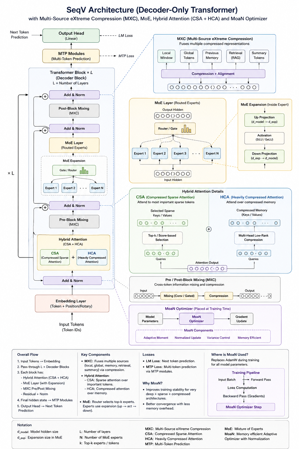
The full-stack view I drew while studying V4: token embedding at the bottom, then a stack of decoder blocks, each wrapping Hybrid Attention and a MoE feed-forward in mHC residual pathways, with Multi-Token Prediction heads at the top and Muon as the training optimizer. The rest of this article is essentially a walk up this diagram, one component at a time. [Notes]
Here is the same block as a data-flow graph — this is the mental model to hold for the whole article:
flowchart TB
    subgraph BLOCK["DeepSeek-V4 Decoder Block (repeated x L)"]
        direction TB
        IN["Hidden states X_l<br/>(n tokens x d)"]

        subgraph RES1["mHC residual pathway #1"]
            direction TB
            MHC1["mHC mix<br/>widen to n_hc streams<br/>B_l on doubly-stochastic manifold"]
        end

        subgraph ATTN["Hybrid Attention sublayer"]
            direction LR
            CSA["CSA branch<br/>compress x m + overlap<br/>Lightning Indexer top-k<br/>MQA on selected blocks"]
            HCA["HCA branch<br/>compress x m' (m' >> m)<br/>no overlap, no selection<br/>MQA on all compressed"]
            CONCAT["Concat"]
            GOP["Grouped Output<br/>Projection (shared)"]
            CSA --> CONCAT
            HCA --> CONCAT
            CONCAT --> GOP
        end

        subgraph RES2["mHC residual pathway #2"]
            direction TB
            MHC2["mHC mix<br/>+ Add & Norm"]
        end

        subgraph FFN["Feed-forward sublayer"]
            direction TB
            MOE["DeepSeekMoE<br/>shared experts + top-K routed<br/>router = sqrt(Softplus(s))"]
        end

        OUT["Hidden states X_l+1<br/>(n tokens x d)"]

        IN --> MHC1 --> ATTN
        GOP --> MHC2 --> MOE --> OUT
    end

    OUT -.->|"stacked hundreds deep,<br/>stability from mHC"| IN

    classDef res fill:#ede7f6,stroke:#5e35b1,stroke-width:2px,color:#000;
    classDef attn fill:#e3f2fd,stroke:#1565c0,stroke-width:2px,color:#000;
    classDef moe fill:#fff3e0,stroke:#ef6c00,stroke-width:2px,color:#000;
    classDef io fill:#e8f5e9,stroke:#2e7d32,stroke-width:2px,color:#000;
    class MHC1,MHC2 res;
    class CSA,HCA,CONCAT,GOP attn;
    class MOE moe;
    class IN,OUT io;
Two sublayers, two mHC pathways, and a hybrid attention core. Now each piece in turn.
III. Manifold-Constrained Hyper-Connections (mHC)
III.1 Why the plain residual is not enough at depth
A standard residual is $X_{l+1} = X_l + F_l(X_l)$ — one identity pathway. Hyper-Connections (HC) generalize this: they widen the residual stream from $\mathbb{R}^d$ to $\mathbb{R}^{n_{hc} \times d}$, giving $n_{hc}$ parallel pathways that the layer can read from and write to. [Notes] The HC update rule is:
\[X_{l+1} = B_l\, X_l + C_l\, F_l\!\left(A_l\, X_l\right)\]Reading the three pieces (this decomposition is the key to understanding mHC): [Notes]
- $A_l \in \mathbb{R}^{1 \times n_{hc}}$ collapses the $n_{hc}$ streams into a single $d$-dimensional input for the layer $F_l$ (so the inner layer is unchanged).
- $B_l \in \mathbb{R}^{n_{hc} \times n_{hc}}$ mixes information among the streams — this is the residual transformation, the dangerous part.
- $C_l \in \mathbb{R}^{n_{hc} \times 1}$ writes the layer’s output back to all streams.
The upside: you decouple residual width ($n_{hc}$) from hidden size ($d$), with low overhead since $n_{hc} \ll d$. The problem: $B_l$ is unconstrained, and stacking many unconstrained mixing matrices is numerically unstable — repeated multiplication can blow the signal up or crush it to zero. [Notes] That is exactly the depth-stability ceiling from Section I.
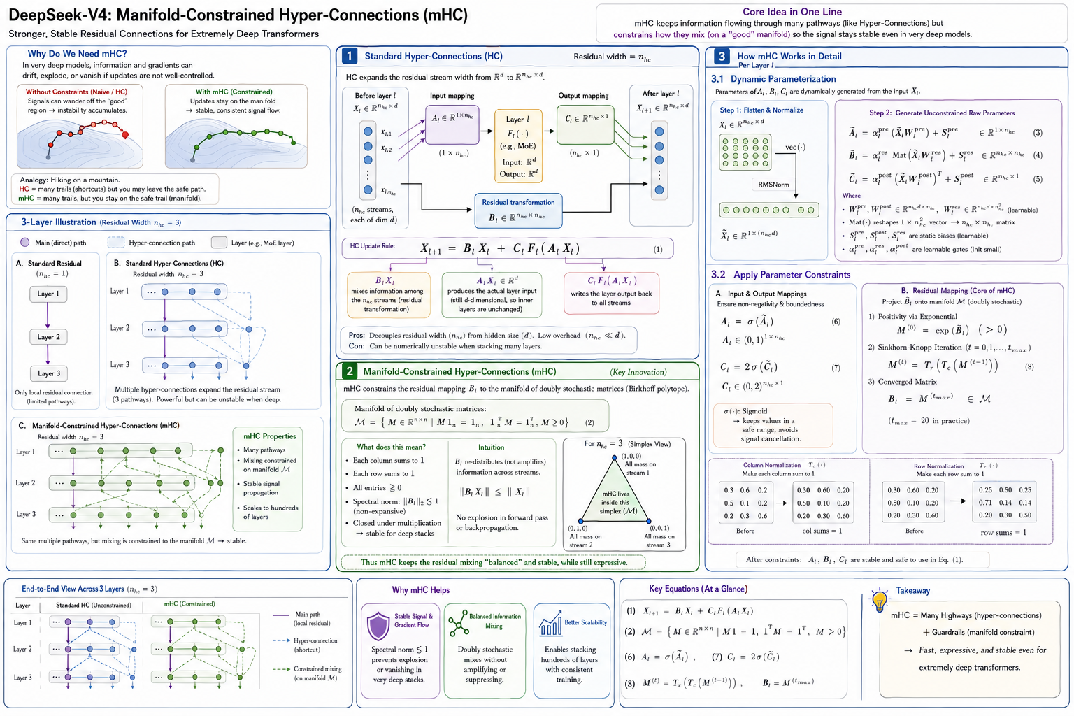
My full mHC breakdown. The left column motivates it with a “hiking on a mountain” analogy — HC gives you many trails (pathways) but you can wander off the safe ridge; mHC keeps the same many trails but adds guardrails (the manifold) so you stay on the stable path. The middle explains the HC update rule; the right shows how the constraint is actually computed. The whole point of the diagram is the one-liner at the top: keep information flowing through many pathways, but constrain how they mix so the signal stays stable even in very deep models. [Notes]
III.2 The constraint: a doubly-stochastic manifold
mHC’s fix is to force $B_l$ to live on the manifold of doubly-stochastic matrices (the Birkhoff polytope):
\[\mathcal{M} = \left\{ M \in \mathbb{R}^{n \times n} \ \middle|\ M \mathbf{1}_n = \mathbf{1}_n,\ \ \mathbf{1}_n^\top M = \mathbf{1}_n^\top,\ \ M \ge 0 \right\}\]In words: every row sums to 1, every column sums to 1, all entries are non-negative. [Notes] Why this specific set? Because a doubly-stochastic matrix redistributes information across streams rather than amplifying it. Its spectral norm satisfies $\lVert B_l \rVert \le 1$ (non-expansive), so:
\[\lVert B_l\, X_l \rVert \ \le\ \lVert X_l \rVert\]The residual mixing can never grow the signal. That single inequality is what buys stability in both the forward pass and backpropagation, which is what lets V4 stack “hundreds of layers” without the signal drifting. [Notes] This is the “guardrail on the mountain trail”: still many pathways, but the mixing is balanced. [Interpretation]
III.3 How the constraint is enforced each step
The raw parameters $\tilde{A}_l, \tilde{B}_l, \tilde{C}_l$ are generated dynamically from the input $X_l$ (flatten, RMSNorm, then learnable projections with small-initialized gates $\alpha$), so mHC is input-dependent, not a fixed set of weights. [Notes] Then each is projected onto its constraint:
- Input/output mappings get squashed to safe ranges: $A_l = \sigma(\tilde{A}_l) \in (0,1)$ and $C_l = 2\,\sigma(\tilde{C}_l) \in (0,2)$, where $\sigma$ is the sigmoid — this keeps values bounded and avoids signal cancellation. [Notes]
- The residual matrix $B_l$ is projected onto $\mathcal{M}$ in two steps: first made positive via $M^{(0)} = \exp(\tilde{B}_l)$, then iterated to double-stochasticity with Sinkhorn-Knopp:
where $T_c(\cdot)$ normalizes each column to sum to 1 and $T_r(\cdot)$ normalizes each row to sum to 1; alternating them converges to a doubly-stochastic matrix. In practice $t_{\max} = 20$ iterations. [Notes] This is cheap because $n_{hc}$ is small.
flowchart LR
    X["Input X_l<br/>(n_hc streams x d)"] --> FLAT["Flatten + RMSNorm<br/>vec(.)"]
    FLAT --> GEN["Generate raw params<br/>via W_pre / W_res / W_post<br/>+ small-init gates alpha"]

    GEN --> RA["A~_l"]
    GEN --> RB["B~_l"]
    GEN --> RC["C~_l"]

    RA --> CA["A_l = sigma(A~_l)<br/>in (0,1)"]
    RC --> CC["C_l = 2 sigma(C~_l)<br/>in (0,2)"]

    subgraph SINK["Project B onto manifold M"]
        direction TB
        POS["M0 = exp(B~_l)<br/>(make positive)"]
        ITER["Sinkhorn-Knopp x t_max=20<br/>M_t = T_row(T_col(M_t-1))"]
        CONV["B_l = M_tmax<br/>doubly-stochastic,<br/>spectral norm <= 1"]
        POS --> ITER --> CONV
    end
    RB --> POS

    CA --> UPD["mHC update:<br/>X_l+1 = B_l X_l + C_l F_l(A_l X_l)"]
    CC --> UPD
    CONV --> UPD

    classDef gen fill:#ede7f6,stroke:#5e35b1,stroke-width:2px,color:#000;
    classDef con fill:#fff3e0,stroke:#ef6c00,stroke-width:2px,color:#000;
    classDef out fill:#e8f5e9,stroke:#2e7d32,stroke-width:2px,color:#000;
    class X,FLAT,GEN,RA,RB,RC gen;
    class CA,CC,POS,ITER,CONV con;
    class UPD out;
The engineering takeaway I keep: mHC = many highways (hyper-connections) + guardrails (the manifold constraint) → fast, expressive, and stable even for extremely deep transformers. [Notes]
IV. Hybrid Attention: CSA and HCA in Parallel
The attention sublayer runs two compressed attention mechanisms side by side and concatenates their outputs:
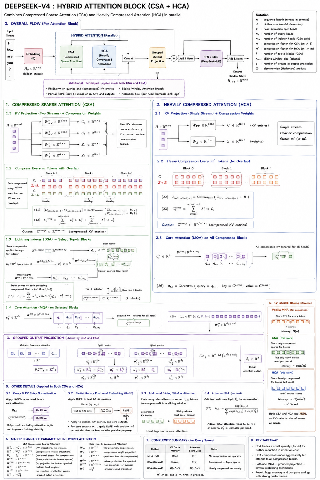
The Hybrid Attention block. Embedding → CSA and HCA in parallel → Concat → Grouped Output Projection → residual add & norm → FFN/MoE. Four techniques are shared inside both branches: RMSNorm on queries and compressed KV entries, partial RoPE (only the last 64 dims), a sliding-window branch for recent tokens, and a per-head learnable attention sink. The design intent is that CSA and HCA are complementary — one keeps quality with moderate compression + selection, the other buys extreme memory savings for very long context. [Notes]
Why two mechanisms instead of one? Because they occupy different points on the same trade-off curve: [Interpretation]
- CSA compresses moderately ($m$), keeps overlap between compressed blocks (so no information falls in the cracks), and is sparse (top-$k$ selection) — this is the quality-preserving path.
- HCA compresses aggressively ($m’ \gg m$), uses no overlap, and is dense over the tiny compressed set — this is the ultra-cheap memory path for very long contexts.
Running both and concatenating lets the model draw from a high-fidelity local/selected view and a heavily-compressed global view in the same block. [Interpretation] In the notes, CSA is used in most layers (better quality) and HCA in some layers (ultra-low memory for long contexts). [Notes]
flowchart TB
    H["Hidden states H<br/>(n x d)"]

    subgraph CSAB["CSA — Compressed Sparse Attention"]
        direction TB
        C1["KV projection: 2 streams<br/>W_KV^a, W_KV^b -> C_a, C_b<br/>W_Z^a, W_Z^b -> Z_a, Z_b"]
        C2["Compress every m tokens<br/>WITH overlap (2m raw per entry)<br/>-> C_comp (n/m x c)"]
        C3["Lightning Indexer (DSA)<br/>index scores I_t,s<br/>Top-k block selector"]
        C4["Core Attention (MQA)<br/>on selected top-k blocks"]
        C1 --> C2 --> C3 --> C4
    end

    subgraph HCAB["HCA — Heavily Compressed Attention"]
        direction TB
        D1["KV projection: 1 stream<br/>W_KV -> C, W_Z -> Z"]
        D2["Heavy compress every m' tokens<br/>NO overlap (m' >> m)<br/>-> C_comp (n/m' x c)"]
        D3["Core Attention (MQA)<br/>on ALL compressed entries"]
        D1 --> D2 --> D3
    end

    H --> C1
    H --> D1
    C4 --> CAT["Concat CSA + HCA outputs"]
    D3 --> CAT
    CAT --> GOP["Grouped Output Projection<br/>(shared): c*n_h -> d in g groups"]
    GOP --> OUT["Attention output o_hat (n x d)"]

    classDef csa fill:#e3f2fd,stroke:#1565c0,stroke-width:2px,color:#000;
    classDef hca fill:#fce4ec,stroke:#c2185b,stroke-width:2px,color:#000;
    classDef shared fill:#fff3e0,stroke:#ef6c00,stroke-width:2px,color:#000;
    classDef io fill:#e8f5e9,stroke:#2e7d32,stroke-width:2px,color:#000;
    class C1,C2,C3,C4 csa;
    class D1,D2,D3 hca;
    class CAT,GOP shared;
    class H,OUT io;
Both branches finish with the same shared Grouped Output Projection and both use MQA (all heads share one compressed $K, V$), so the KV cache is shared across heads. [Notes] Now each branch in detail.
V. Compressed Sparse Attention (CSA)
CSA’s high-level idea: compress the KV cache by a factor $m$, select the top-$k$ compressed entries for each query via a Lightning Indexer, then run core attention in MQA fashion. [Notes]
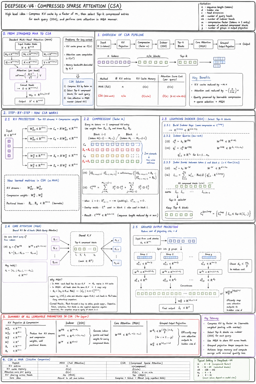
My step-by-step CSA breakdown. The pipeline is: KV projection (two streams) → compression with overlap → Lightning Indexer (top-$k$ selection) → MQA core attention → grouped output projection. The comparison table at the bottom is the payoff: MHA keeps $n$ KV entries at $O(n)$ memory and $O(n)$ attention cost; CSA keeps $n/m$ entries at $O(n/m)$ memory and $O(k)$ attention cost with $k \ll n/m \ll n$. [Notes]
V.1 Compression with overlap
CSA projects the hidden states into two KV streams ($C_a, C_b$ via $W_{KV}^a, W_{KV}^b$) and two compression-weight streams ($Z_a, Z_b$ via $W_Z^a, W_Z^b$). Two streams give diversity; the $Z$ streams produce the compression scores. [Notes] Every $m$ tokens are pooled into one compressed entry, but with overlap — each compressed entry $C_i^{comp}$ draws on $2m$ raw KV entries (block $i-1$ and block $i$), so information near a block boundary is never lost. The pooling weights are a row-wise softmax over the $Z$ scores plus a learnable positional bias, and the compressed entry is their weighted sum:
\[C_i^{comp} = \sum_{j=m_i}^{m_{(i+1)}-1} S_j^{a} \odot C_j^{a} \ +\ \sum_{j=m_{(i-1)}}^{m_i - 1} S_j^{b} \odot C_j^{b}\]The result is $C^{comp} \in \mathbb{R}^{n/m \times c}$ — the sequence length is cut by roughly $m\times$. [Notes] ($\odot$ is element-wise product; $S$ are the softmax pooling weights over $Z + \text{bias}$.)
V.2 The Lightning Indexer (DSA): top-$k$ selection
Compression alone gives $n/m$ entries; sparsity comes from selecting only the $k$ most relevant compressed blocks per query. The Lightning Indexer builds low-rank indexer keys $K^{I,comp} \in \mathbb{R}^{n/m \times c_I}$ (same compression applied to keys) and low-rank indexer queries $q_t^I$, then scores each preceding compressed block $s$ for query token $t$:
\[I_{t,s} = \sum_{h=1}^{n_{ih}} w_{t,h}^{I}\, \cdot\, \text{ReLU}\!\left(q_{t,h}^{I} \cdot K_s^{I,comp}\right)\]The sum runs over $n_{ih}$ indexer heads, each with a learned weight $w_{t,h}^I$; the ReLU keeps only positive matches. A top-$k$ selector then keeps the highest-scoring blocks: $C_t^{Sprs,comp} = { C_s^{comp} \mid I_{t,s} \in \text{Top-}k(I_{t,:}) }$. [Notes] The indexer is deliberately low-rank and cheap — it is a fast pre-filter whose only job is to pick which $k$ blocks the expensive core attention will actually look at. [Interpretation]
V.3 Core attention and grouped output
Core attention then runs only over the selected $k$ blocks, in MQA form — all heads share the same compressed $K, V$, so the cache holds one copy instead of $n_h$. [Notes] Finally the Grouped Output Projection maps the concatenated head outputs ($c \cdot n_h$ dimensions) back to $d$: it splits the heads into $g$ groups, projects each group with a smaller matrix ($d_g < c\,n_h / g$), and concatenates — cutting the cost of the output projection. [Notes]
The cost ledger, which is the whole reason CSA exists: [Notes]
| Method | KV entries | KV-cache memory | Attention cost / query |
|---|---|---|---|
| MHA (full) | $n$ | $O(n)$ | $O(n)$ |
| CSA | $n/m$ | $O(n/m)$ | $O(k)$, with $k \ll n/m \ll n$ |
Typical settings in the notes: $m = 4\text{–}8$, $k = 16\text{–}64$, $n_{ih} = 128\text{–}256$, $n_h = 4\text{–}8$, $g = 8\text{–}16$. [Notes]
flowchart LR
    H["H (n x d)"] --> KV["KV proj: 2 streams<br/>C_a,C_b + Z_a,Z_b"]
    KV --> COMP["Compress x m WITH overlap<br/>C_comp (n/m x c)"]
    COMP --> IDX["Lightning Indexer<br/>I_t,s = sum_h w ReLU(q . K)"]
    IDX --> TOPK["Top-k selector<br/>keep k blocks"]
    TOPK --> CORE["Core Attention (MQA)<br/>over k selected blocks"]
    CORE --> GOP["Grouped Output Projection<br/>g groups, d_g < c*n_h/g"]
    GOP --> O["o_hat (n x d)"]

    classDef step fill:#e3f2fd,stroke:#1565c0,stroke-width:2px,color:#000;
    classDef sel fill:#fff3e0,stroke:#ef6c00,stroke-width:2px,color:#000;
    classDef io fill:#e8f5e9,stroke:#2e7d32,stroke-width:2px,color:#000;
    class KV,COMP,CORE,GOP step;
    class IDX,TOPK sel;
    class H,O io;
VI. Heavily Compressed Attention (HCA)
HCA is CSA’s aggressive sibling. It compresses much harder ($m’ \gg m$), uses no overlap, and does not do sparse selection — every query attends to all compressed KV entries (MQA). [Notes]
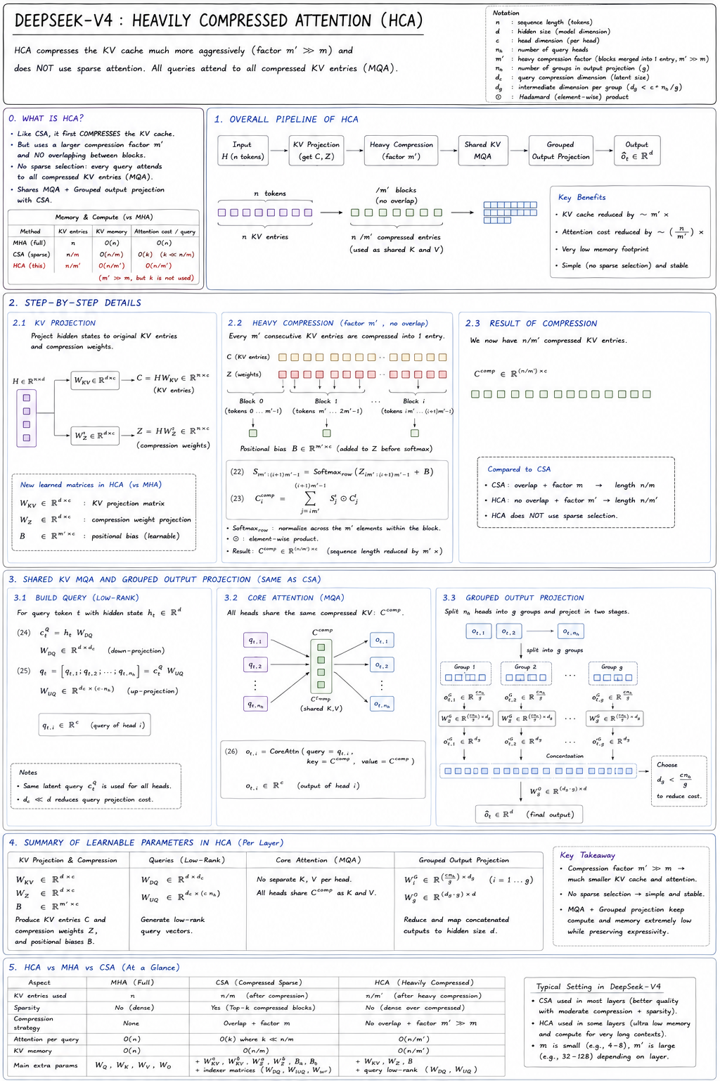
My HCA breakdown. Single KV stream (vs CSA’s two), heavy compression factor $m’$ with no overlap, and — crucially — no top-$k$ selection: because the compressed set is already tiny ($n/m’$ entries), you can afford to attend to all of it densely. The comparison box makes the contrast explicit: CSA is *overlap + factor $m$ + top-$k$; HCA is no overlap + factor $m’$ + dense.* [Notes]
The compression is a single-stream version of CSA’s: project to KV entries $C$ and compression weights $Z$, then pool every $m’$ non-overlapping tokens with a row-wise softmax over $Z$ plus positional bias:
\[C_i^{comp} = \sum_{j = m'i}^{m'(i+1)-1} S_j^{comp} \odot C_j, \qquad C^{comp} \in \mathbb{R}^{n/m' \times c}\]Then core attention is dense over that tiny set — all heads share it (MQA): [Notes]
\[o_{t,i} = \text{CoreAttn}\!\left(\text{query} = q_{t,i},\ \text{key} = C^{comp},\ \text{value} = C^{comp}\right)\]Because $m’$ is large (the notes give $m’ = 32\text{–}128$), the KV cache and attention cost are both $O(n/m’)$ — a very low memory footprint, and dead simple because there is no indexer or selection to maintain. [Notes] That simplicity is the point: HCA is the stable, cheap “background” attention that handles very long context, while CSA does the high-fidelity work. [Interpretation]
Putting the three side by side (the summary table from the notes): [Notes]
| Aspect | MHA (full) | CSA (sparse) | HCA (heavy) |
|---|---|---|---|
| KV entries used | $n$ | $n/m$ | $n/m’$ |
| Sparsity | no | yes (top-$k$) | no (dense over compressed) |
| Compression | none | overlap + factor $m$ | no overlap + factor $m’ \gg m$ |
| Attention / query | $O(n)$ | $O(k)$ | $O(n/m’)$ |
| KV memory | $O(n)$ | $O(n/m)$ | $O(n/m’)$ |
VII. DeepSeekMoE with a $\sqrt{\text{Softplus}}$ Router
The feed-forward sublayer keeps the DeepSeekMoE design inherited from V2/V3 — a set of always-on shared experts plus a large pool of fine-grained routed experts, of which only the top-$K$ fire per token. What changes in V4 is the routing activation.
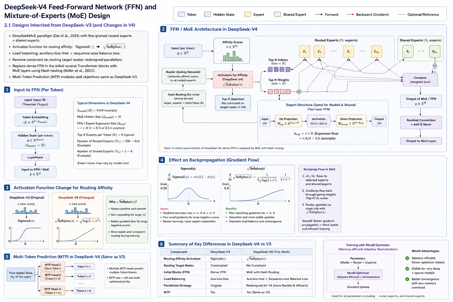
My FFN/MoE breakdown. The router computes affinity scores over $N_r$ routed experts; the top-$K$ (K = 8 typical) are combined with $N_s$ shared experts (always on) via a weighted sum, then added back through the residual. Each expert is a two-layer FFN with up-projection, SiLU/GeLU, and down-projection. Two V4-specific twists appear here: the $\sqrt{\text{Softplus}}$ routing activation and Hash routing in the initial several blocks. [Notes]
VII.1 Why $\sqrt{\text{Softplus}}$ instead of Sigmoid
V3 computed routing affinity with a Sigmoid. V4 replaces it with:
\[\text{affinity} = \sqrt{\text{Softplus}(s)} = \sqrt{\log\!\left(1 + e^{s}\right)}\]The reason is entirely about gradient flow. A sigmoid saturates: for $s \ll 0$ or $s \gg 0$ its derivative $\sigma(s)(1-\sigma(s)) \to 0$, so experts with large-negative scores receive almost no gradient and are rarely explored — routing gets stuck. [Notes] Compare the derivatives:
\[\frac{d}{ds}\,\sigma(s) = \sigma(s)\bigl(1 - \sigma(s)\bigr) \qquad\text{vs}\qquad \frac{d}{ds}\sqrt{\text{Softplus}(s)} = \frac{1}{2\sqrt{\log(1+e^{s})}}\cdot\frac{1}{1 + e^{-s}}\]| The $\sqrt{\text{Softplus}}$ form is **always positive, smooth, and non-saturating for large $ | s | $: its gradient does **not vanish for large-negative scores, so under-used experts keep getting a learning signal. [Notes] The practical effect the notes call out: smoother, more stable routing updates, better expert exploration, and improved load balance and convergence. [Interpretation] |
VII.2 The rest of the MoE, and what carries over from V3
The other V4 MoE choices, from the notes: [Notes]
- Load balancing: auxiliary-loss-free (V3’s bias trick) plus a sequence-wise balance loss.
- No constraint on routing target nodes, with a redesigned, more flexible parallelism strategy.
- Hash routing in the initial several blocks: the first few transformer blocks replace the dense FFN with an MoE whose routing is a deterministic hash of the token ID (
target_experts = Hash(TokenID)) rather than a learned router. - MTP is unchanged from V3 (see next section).
- Expert dimensions (example): $d_{\text{model}} = H = 6144$, expansion $d_{\text{esp}} = r \cdot H$ with $r \approx 8/3 \text{–} 3.5$, top-$K = 8$, $N_r = 256\text{–}512$ routed experts, $N_s = 1\text{–}8$ shared experts.
During backprop, $\partial L / \partial y$ flows to the selected routed experts and the shared experts, then back through the gating weights to the router, which is updated via the chain rule through $\sqrt{\text{Softplus}}$ — and because that gradient never dies, the router keeps improving. [Notes]
flowchart TB
    X["Token hidden x_hat (H)"] --> R["Router (gating)<br/>affinity scores s (N_r)"]
    R --> ACT["Activation<br/>sqrt(Softplus(s))"]
    ACT --> SEL["Top-K selection<br/>(K=8, no target-node constraint)"]

    SEL --> E1["Routed Expert i<br/>(2-layer FFN:<br/>Up -> SiLU -> Down)"]
    SEL --> E2["Routed Expert j"]
    X --> S1["Shared Expert(s)<br/>(always on)"]

    E1 --> COMB["Weighted Sum"]
    E2 --> COMB
    S1 --> COMB
    COMB --> Y["MoE output y (H)"]
    Y --> ADD["Residual add & norm (mHC)"]

    HASH["Hash routing<br/>(initial blocks only):<br/>experts = Hash(TokenID)"] -.->|"replaces learned router<br/>in first few blocks"| R

    classDef route fill:#fff3e0,stroke:#ef6c00,stroke-width:2px,color:#000;
    classDef exp fill:#e3f2fd,stroke:#1565c0,stroke-width:2px,color:#000;
    classDef shared fill:#e8f5e9,stroke:#2e7d32,stroke-width:2px,color:#000;
    class R,ACT,SEL,HASH route;
    class E1,E2 exp;
    class S1,COMB,Y,ADD,X shared;
VIII. Multi-Token Prediction (MTP)
MTP in V4 is the same as in V3: alongside the main next-token head, additional MTP modules predict further-out tokens (next, next-next, …), and the MTP loss is optimized jointly with the standard language-modeling loss. [Notes] This densifies the training signal (more supervision per position) and, kept at inference, enables speculative decoding for faster generation.
Because this is unchanged, I will not re-derive it here — the full treatment (the sequentially-causal chain, the shared trunk, the acceptance-rate speedup) is in the DeepSeek-V3 dissection. [Interpretation]
IX. The Muon Optimizer
V4’s fourth pillar is not architectural — it is the training algorithm. Muon is a matrix-aware optimizer: instead of treating each parameter as a scalar with a scalar learning rate (Adam/SGD), it treats each weight $W \in \mathbb{R}^{n \times m}$ as a 2D object and preconditions the update using second-order structure. [Notes]
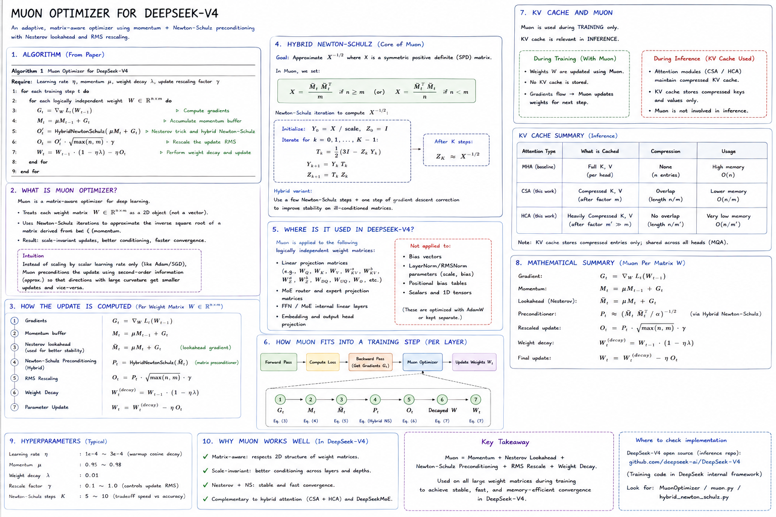
My Muon breakdown. The core is a hybrid Newton-Schulz iteration that approximates $X^{-1/2}$ (the inverse square root of a matrix built from the gradient), which acts as a preconditioner — directions with large curvature get smaller updates and vice versa. The notes list exactly where it is applied (2D matrices) and where it is not (biases, norms, scalars), and note it is a training-only optimizer with no role in inference. [Notes]
IX.1 The update, step by step
For each 2D weight matrix, per training step: [Notes]
\[G_t = \nabla_W L_t(W_{t-1}) \qquad M_t = \mu M_{t-1} + G_t\] \[O'_t = \text{HybridNewtonSchulz}\!\left(\mu M_t + G_t\right) \qquad O_t = O'_t \cdot \sqrt{\max(n, m)} \cdot \gamma\] \[W_t = W_{t-1}\,(1 - \eta\lambda) \ -\ \eta\, O_t\]Reading it: $M_t$ is the momentum buffer; feeding $\mu M_t + G_t$ into the preconditioner is the Nesterov lookahead (use a gradient estimate one step ahead); the $\sqrt{\max(n,m)}\cdot\gamma$ factor is RMS rescaling that keeps the update magnitude sane regardless of matrix shape; and the final line applies decoupled weight decay ($1-\eta\lambda$) before the gradient step. [Notes]
IX.2 The hybrid Newton-Schulz core
The preconditioner approximates $X^{-1/2}$ for the symmetric positive-definite matrix
\[X = \frac{\tilde{M}_t\, \tilde{M}_t^\top}{m}\ \ (n \ge m) \qquad\text{or}\qquad X = \frac{\tilde{M}_t^\top\, \tilde{M}_t}{n}\ \ (n < m)\]using an iteration that needs only matrix multiplies (no eigendecomposition): initialize $Y_0 = X/\text{scale}$, $Z_0 = I$, then for $k = 0,1,\dots,K-1$
\[T_k = \tfrac{1}{2}\bigl(3I - Z_k Y_k\bigr), \qquad Y_{k+1} = Y_k T_k, \qquad Z_{k+1} = T_k Z_k\]after $K$ steps $Z_K \approx X^{-1/2}$. [Notes] The “hybrid” variant adds a gradient-descent correction step to stay stable on ill-conditioned matrices. In practice $K = 5\text{–}10$ steps (a speed/accuracy trade-off). [Notes]
IX.3 What Muon touches — and what it doesn’t
Muon is applied to the 2D weight matrices: the attention projections (all the $W_Q, W_K, W_V, W_{KV}, W_Z, W_{DQ}, W_{UQ}, W_O$ of CSA/HCA), the MoE router and expert projections, the FFN linear layers, and the embedding/output head. It is not applied to biases, LayerNorm/RMSNorm scale-and-shift parameters, positional-bias tables, or any scalar/1D tensor — those stay on AdamW. [Notes] And it is training-only: the KV-cache compression (CSA/HCA) is an inference-time concern; Muon plays no part there. [Notes]
flowchart LR
    FWD["Forward pass"] --> LOSS["Compute loss L"]
    LOSS --> GRAD["Backward:<br/>G_t = grad_W L"]
    GRAD --> MOM["Momentum:<br/>M_t = mu M_t-1 + G_t"]
    MOM --> NES["Nesterov lookahead:<br/>mu M_t + G_t"]
    NES --> NS["Hybrid Newton-Schulz:<br/>approx X^-1/2 (K=5-10 iters)"]
    NS --> RMS["RMS rescale:<br/>x sqrt(max(n,m)) x gamma"]
    RMS --> WD["Weight decay + update:<br/>W_t = W_t-1(1-eta lambda) - eta O_t"]
    WD --> NEXT["Updated weights"]

    classDef step fill:#ede7f6,stroke:#5e35b1,stroke-width:2px,color:#000;
    classDef core fill:#fff3e0,stroke:#ef6c00,stroke-width:2px,color:#000;
    classDef io fill:#e8f5e9,stroke:#2e7d32,stroke-width:2px,color:#000;
    class MOM,NES,RMS,WD step;
    class NS core;
    class FWD,LOSS,GRAD,NEXT io;
Hyperparameters from the notes: learning rate $\eta = 1\text{e-}4$ to $3\text{e-}4$ (warmup + cosine decay), momentum $\mu = 0.95\text{–}0.98$, weight decay $\lambda = 0.01$, rescale factor $\gamma = 0.1\text{–}1.0$, Newton-Schulz steps $K = 5\text{–}10$. [Notes] Why it fits V4: matrix-aware and scale-invariant updates give better conditioning across the many layers that mHC now lets you stack, with stable, fast convergence — complementary to the hybrid attention + DeepSeekMoE design. [Interpretation]
X. How It All Fits Together
The four pillars are not independent — they reinforce each other. [Interpretation]
- mHC removes the depth ceiling, so you can stack more layers…
- …which is only affordable because Hybrid Attention made each layer’s attention sub-quadratic ($O(n/m)$ memory, $O(k)$ or $O(n/m’)$ compute)…
- …and DeepSeekMoE keeps the per-token compute flat even as total parameters grow, with the $\sqrt{\text{Softplus}}$ router keeping all those experts actually trainable…
- …while Muon keeps the whole tall, wide, sparse model well-conditioned during training, and MTP squeezes more signal out of every token.
Put differently: V2 made the model fit in memory, V3 made it cheap to train, and V4 makes it deep and long-context without either of those regressing. [Interpretation]
XI. Trade-offs and Limitations
Being honest about the costs, several of which the notes make explicit and some of which are my reading: [Interpretation]
- Compression can drop information. CSA’s overlap and top-$k$ selection are bets that the discarded blocks did not matter for a given query. For tasks needing exact recall of an arbitrary distant token (needle-in-a-haystack style), heavy compression — especially HCA at $m’ = 128$ — is a real risk. The two-branch design is partly insurance against this. [Interpretation]
- The Lightning Indexer is another moving part. Top-$k$ selection is only as good as the indexer’s scores; a bad pre-filter silently starves core attention of the right blocks, and the indexer adds its own parameters and compute. [Interpretation]
- mHC adds per-step cost. Twenty Sinkhorn-Knopp iterations per mHC block, every forward pass, is not free — it is cheap only because $n_{hc}$ is small. [Derived]
- Muon’s Newton-Schulz costs matrix multiplies. $K = 5\text{–}10$ iterations of matrix products per 2D weight per step is more per-step optimizer work than AdamW; the bet is that better conditioning pays it back in fewer steps and higher stability. [Interpretation]
- This is an architecture study, not a benchmarked result here. I have deliberately not attached accuracy or throughput numbers, because my notes are about mechanism, not a reproduction of published evaluations. Treat the “$m\times$ / $O(n/m)$” claims as the design intent, and verify against the official release before quoting figures. [Interpretation]
XII. Engineer’s Takeaway
If I compress DeepSeek-V4 to a few sentences: it is the DeepSeek recipe finally attacking the $O(n^2)$ attention term and the depth-stability ceiling at the same time. [Interpretation] Hybrid Attention says you do not need to compare every token to every token — compress, then select — and hedges its compression with two branches at different fidelities. mHC says widen the residual into many pathways, but keep the mixing on a manifold where nothing can blow up, which is what makes stacking that many layers safe. The $\sqrt{\text{Softplus}}$ router and Muon are the quieter enablers: keep every expert learnable, and keep every matrix well-conditioned.
The pattern worth stealing, regardless of DeepSeek: when a cost is quadratic, do not optimize the constant — change what you compute. Compress the thing you are attending over, then spend your attention budget only where an cheap indexer says it will matter. [Interpretation]
Related Reading
- DeepSeek-V3: Auxiliary-Loss-Free MoE, MTP, and FP8 Training — the direct predecessor; V4 inherits DeepSeekMoE and MTP from here and changes the router activation.
- DeepSeek-V2: Mixture-of-Experts and Multi-head Latent Attention — where the KV-cache-compression lineage (MLA) that Hybrid Attention descends from begins.
- DeepSeek-R1: Incentivizing Reasoning via Reinforcement Learning — the reasoning line built on the same base models.