Why This Paper Matters
When BERT appeared in October 2018, it did not merely set new benchmark records. It fundamentally shifted what the research community believed was achievable through pre-training alone. Before BERT, the dominant assumption was that a pre-trained language model was a starting point — a rough feature extractor that you needed to heavily engineer around for each specific task. After BERT, that assumption collapsed. A single pre-trained model, fine-tuned with one extra linear layer, beat purpose-built architectures across eleven different NLP benchmarks simultaneously.
To understand why that is remarkable, you need to understand what the field looked like in mid-2018 and precisely what problem BERT solved.
The Unidirectionality Problem
Every pre-trained language model before BERT had the same fundamental limitation: it read text in one direction. OpenAI GPT processed sequences left-to-right — when processing the word “bank” in “I went to the bank to deposit money,” GPT could see all the words before it but none after it. ELMo attempted to address this by running two separate language models — one left-to-right and one right-to-left — and concatenating their representations. But this shallow concatenation is not the same as truly reading both directions at the same time. Each direction is trained independently; the interaction between left and right context happens only at the very end, at the representation level, not during the actual computation of each token’s meaning.
This unidirectionality is not a quirk — it is a consequence of how autoregressive language models are trained. If you train a model to predict the next word, then by definition the model cannot look at future words during training, because those are the targets. The design of the training objective enforces unidirectionality.
BERT breaks this constraint with a different training objective entirely: instead of predicting the next word, predict a masked word using context from both sides simultaneously. This is the core conceptual move of the paper, and everything else follows from it.
What BERT Changed
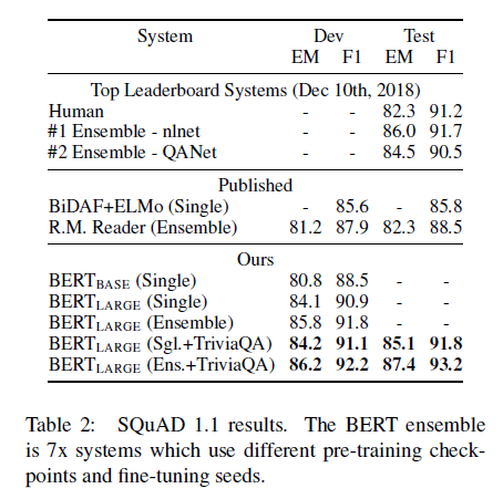
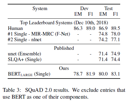
The downstream cascade was immediate. BERT pushed the GLUE benchmark — a multi-task NLP evaluation suite — from 72.8 to 80.5 in one paper. It improved SQuAD v1.1 question answering F1 from 91.7 to 93.2, surpassing human-level ensemble systems. It pushed SQuAD v2.0 F1 from 78.0 to 83.1. These were not incremental gains. They represented a step-change that made it clear that representation quality from pre-training was the dominant factor in NLP performance — more important than task-specific architecture design.
BERT also made transfer learning the standard paradigm for NLP in the same way ImageNet pre-training had become standard for computer vision. Every significant NLP model that followed — RoBERTa, ALBERT, XLNet, DistilBERT, and the encoder-based components of T5 — is a direct descendant or deliberate variation of BERT.
The Pre-BERT Landscape: Why Unidirectionality Was Limiting
Before engaging with BERT’s architecture, it is worth understanding the two approaches it was built in reaction to.
Feature-Based Approaches: ELMo
ELMo (Peters et al., 2018) produced contextualised word representations by running two independent language models — one reading left-to-right, one right-to-left — and concatenating their hidden states at each token position. The resulting representations were then used as additional input features fed into task-specific architectures.
The key limitation is in the word “shallow.” The two directions are never trained to interact. A left-to-right LSTM processes “Paris is the capital of France” by building up a hidden state from left to right, and a right-to-left LSTM processes the same sentence from right to left. For the word “capital,” the left context (“Paris is the”) and the right context (“of France”) are encoded by two completely separate models with no shared computation. Concatenating these two vectors gives you information from both directions, but not a representation that was formed by truly attending to both simultaneously.
Fine-Tuning Approaches: OpenAI GPT
GPT (Radford et al., 2018) demonstrated that a Transformer trained left-to-right on a large corpus, then fine-tuned on task-specific data, achieved strong results across multiple NLP tasks. The architecture is clean: pre-train a large autoregressive decoder, then add a small task-specific head and fine-tune everything end-to-end.
But the left-to-right constraint is a hard architectural constraint, not just a training choice. In GPT’s self-attention layers, every token can only attend to tokens that came before it — this is enforced by a causal attention mask that zeros out all attention weights to future positions. This mask is not removable without retraining from scratch. For tasks like question answering, where the question appears after the passage in the concatenated input, the model processes the passage without being able to “see” the question it will need to answer. This is fundamentally sub-optimal.
BERT’s insight: use the Transformer encoder (which has no causal masking) and design a training objective that does not require left-to-right prediction. The encoder’s bidirectional attention is already there — you just need a training task that can exploit it.
The Core Idea: Masked Language Modelling
The conceptual move that makes BERT possible is simple to state and non-obvious to arrive at: if you want to train a bidirectional model, mask the targets during training so the model cannot simply copy them.
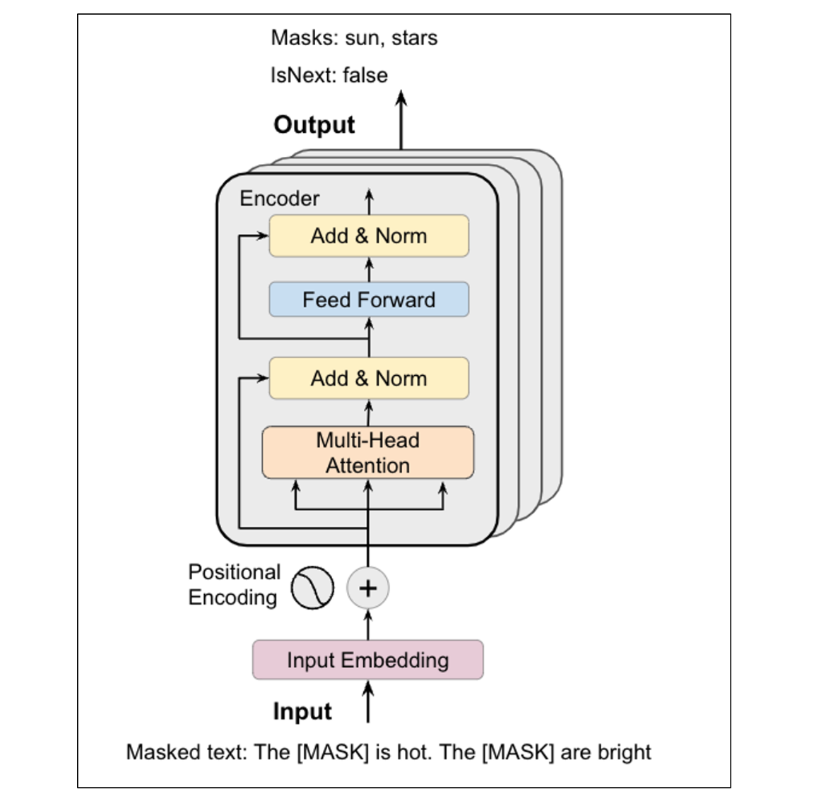
In a standard autoregressive model, the reason you cannot look at future tokens is that the target word is always the next unmasked token — if you could see it, you would just copy it and learn nothing. BERT changes the training setup: randomly hide 15% of tokens in the input, and ask the model to predict what the hidden tokens were. Now the model can attend to both the tokens before and after the masked position, because the masked token itself has been removed from the input. The model cannot cheat by looking at the target — the target has been replaced with a [MASK] placeholder.
This is called the Cloze task, described by Taylor in 1953 as a reading comprehension tool where blanks are inserted into text. BERT’s MLM is a neural, large-scale version of the same idea.
The 80-10-10 Masking Strategy
A practical problem arises immediately: the [MASK] token is an artifact of pre-training that never appears during fine-tuning on real tasks. If the model is trained to repair [MASK] tokens, but fine-tuned on tasks with no [MASK] tokens, there is a distribution mismatch between pre-training and fine-tuning.
BERT addresses this with a three-way masking strategy for the 15% of selected tokens:
- 80% of the time: Replace with
[MASK]— the standard case. - 10% of the time: Replace with a random word from the vocabulary.
- 10% of the time: Keep the original word unchanged.
The effect of this strategy is subtle but important. Because the model never knows whether a given token was masked, replaced with a random word, or kept unchanged, it cannot “switch off” when it does not see a [MASK] token. It must maintain a contextual representation of every token at all times, on the chance that it might be asked to predict it. This forces the encoder to build rich, general-purpose representations of every position — exactly what you want for downstream tasks.
The random replacement accounts for only 10% of selected tokens (so 1.5% of all tokens overall), which is too small to meaningfully harm language understanding, but large enough to prevent the model from ignoring all non-masked tokens during prediction.
Architecture
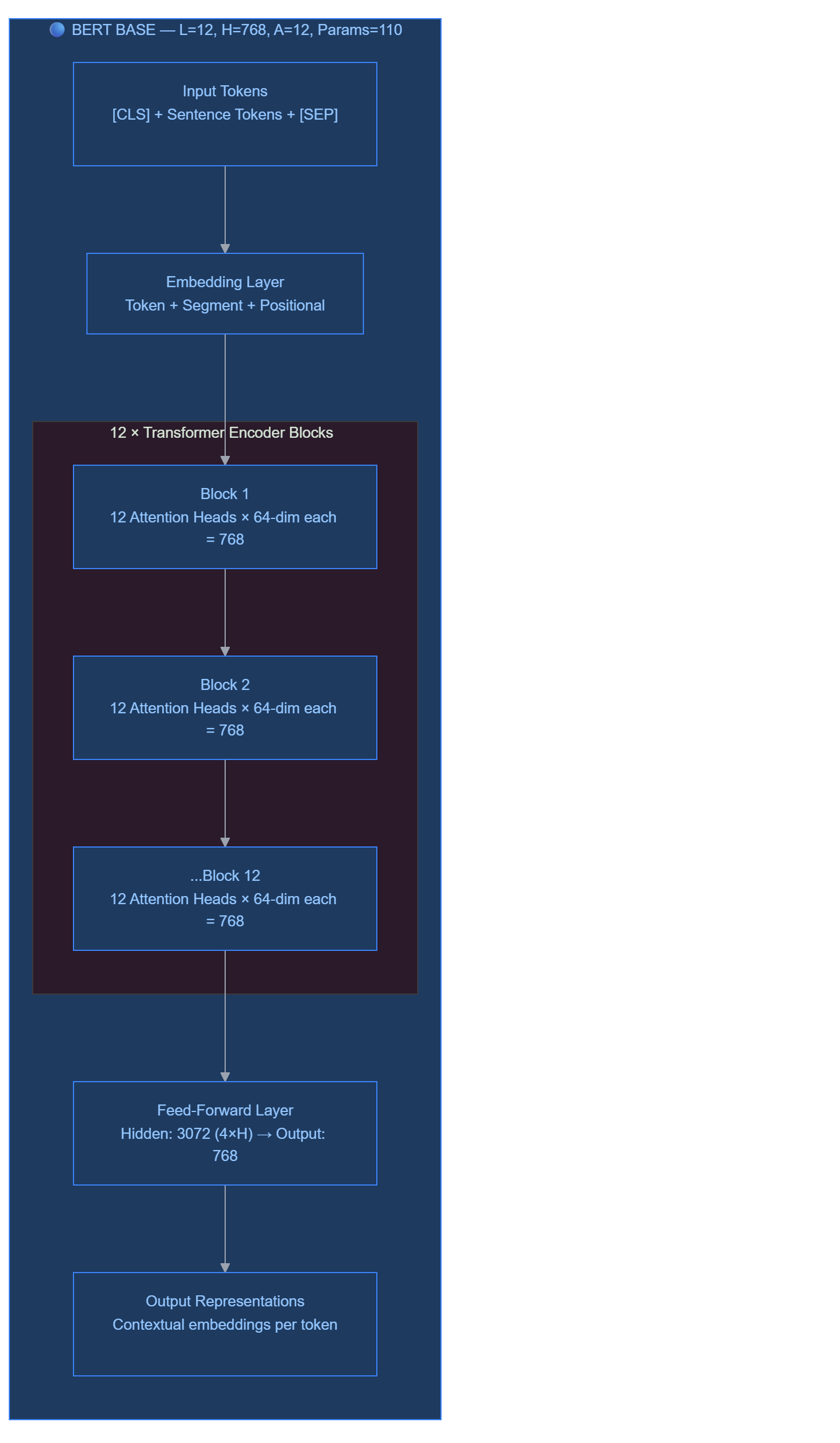
BERT is a multi-layer bidirectional Transformer encoder. It uses only the encoder stack from the original Transformer (Vaswani et al., 2017) — there is no decoder. Every token attends to every other token in every layer, with no causal masking.
BERT Base vs BERT Large
Two variants were released, parameterised by three numbers:
| Config | BERT Base | BERT Large |
|---|---|---|
| Layers (L) | 12 | 24 |
| Hidden size (H) | 768 | 1024 |
| Attention heads (A) | 12 | 16 |
| Head dimension | 768 ÷ 12 = 64 | 1024 ÷ 16 = 64 |
| FFN inner dimension | 4 × 768 = 3,072 | 4 × 1024 = 4,096 |
| Total parameters | 110M | 340M |
Two observations that matter:
Head dimension is always 64. Whether you use 12 heads or 16 heads, the per-head dimensionality stays constant. What scales is the number of heads and the number of layers, not the per-head computation. This is a deliberate design choice — the per-head capacity is kept fixed while the model’s breadth (number of heads) and depth (number of layers) increase.
BERT Base was sized to match OpenAI GPT. This was intentional: the authors wanted a fair comparison with the existing state of the art. When BERT Base outperforms GPT on every task despite having the same parameter count, the architecture (bidirectional encoder vs. causal decoder) is the only variable that changed.
BERT vs GPT: The Architectural Difference
| BERT | GPT | |
|---|---|---|
| Attention type | Full bidirectional self-attention | Causal (left-only) self-attention |
| What each token sees | All tokens — left AND right | Only tokens to its left |
| Training objective | Masked Language Model (fill in blanks) | Autoregressive LM (predict next token) |
| Best for | Understanding tasks (classification, QA, NER) | Generation tasks (text completion) |
| Architecture component | Transformer encoder only | Transformer decoder only |
This is not a “BERT is better” comparison — GPT’s causal masking is a necessary design for text generation. But for tasks where you need to understand the meaning of a complete sentence or passage, full bidirectional context is strictly more powerful.
Input Representation
One of BERT’s most important design decisions is its unified input format. NLP tasks have very different input shapes: some need a single sentence (sentiment analysis, NER), others need pairs of sentences (question answering, natural language inference). BERT handles all of these with the same architecture by encoding everything as a single token sequence.
Special Tokens: [CLS] and [SEP]
Two special tokens structure every BERT input:
| Token | Purpose |
|---|---|
[CLS] |
Always the first token. Its final hidden state acts as the aggregate representation of the entire input — used for classification tasks. |
[SEP] |
Separator between sentences. Also marks the end of the final sentence. |
Single sentence input:
[CLS] The cat sat on the mat [SEP]
Sentence pair input:
[CLS]  Where  is  Paris ?  [SEP]  Paris  is  in  France .  [SEP]
       ◄────── Sentence A ───────►  ◄──────── Sentence B ──────────►
The model handles both formats identically — the only difference is the segment embedding (described below) that tells the model which sentence each token belongs to.
Three Embeddings, Summed
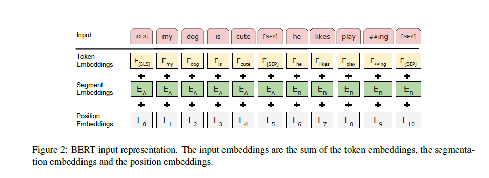
Every token’s input vector is the sum of three learned embeddings:
| Embedding | What it encodes |
|---|---|
| Token embedding | The meaning of the word itself, from a 30,000-token WordPiece vocabulary |
| Segment embedding | Which sentence this token belongs to — E_A for Sentence A, E_B for Sentence B |
| Position embedding | Where in the sequence this token sits (learned, not sinusoidal like the original Transformer) |
Input vector for token t = TokenEmb(t) + SegmentEmb(sentence) + PositionEmb(position)
One important difference from the original Transformer: BERT uses learned positional embeddings rather than fixed sinusoidal encodings. In practice, both approaches work, but learned embeddings offer slightly more flexibility on the specific sequence lengths seen during pre-training.
The [CLS] token is deliberately placed at position 0 with no inherent lexical meaning — it is designed to aggregate information across the entire sequence through self-attention across all 12 or 24 layers. By the final layer, its embedding has attended to every other token at every layer and accumulated a global summary of the input.
Pre-Training Tasks
BERT is pre-trained simultaneously on two unsupervised tasks using a massive unlabelled corpus (BooksCorpus, 800M words + English Wikipedia, 2.5B words).
Task 1: Masked Language Model (MLM)
The procedure:
- Tokenise the input sentence.
- Randomly select 15% of tokens.
- For each selected token, apply the 80-10-10 strategy:
- 80% → replace with
[MASK] - 10% → replace with a random vocabulary token
- 10% → keep unchanged
- 80% → replace with
- Run the full bidirectional encoder.
- At each masked position, use the final hidden state to predict the original token via a softmax over the vocabulary.
Training examples:
Input:   [CLS] The cat [MASK] on the mat [SEP]
Target:  Predict → "sat"

Input:   [CLS] The [MASK] barked loudly at the stranger [SEP]
Target:  Predict → "dog"

Input:   [CLS] [MASK] is the capital of France [SEP]
Target:  Predict → "Paris"
The critical property: to correctly predict [MASK], the model must understand the full context — left and right — simultaneously. Predicting “sat” requires understanding “The cat” and “on the mat” together. This forces deep contextual representations in every layer.
The masked language model only predicts the 15% of masked tokens, not all tokens. This is less efficient than standard language model pre-training (which gets a training signal from every token), but the bidirectional context more than compensates in representation quality.
Task 2: Next Sentence Prediction (NSP)
Many downstream tasks — question answering, natural language inference — require understanding the relationship between two sentences, not just their individual meanings. Standard language modelling gives no training signal for cross-sentence relationships. NSP provides this signal directly.
During pre-training, BERT is given pairs of sentences (A, B):
- 50% of the time: B genuinely follows A in the original document (labelled
IsNext) - 50% of the time: B is a random sentence from the corpus (labelled
NotNext)
Training examples:
IsNext:
[CLS] The dog barked all night. [SEP] The neighbours filed a complaint. [SEP]

NotNext:
[CLS] The dog barked all night. [SEP] Photosynthesis requires sunlight. [SEP]

IsNext (QA-style):
[CLS] Where is the Eiffel Tower? [SEP] The Eiffel Tower is located in Paris, France. [SEP]
The [CLS] token’s final hidden state is fed into a binary classifier (a single linear layer) that predicts IsNext / NotNext. This trains the model to understand cross-sentence coherence — a signal that proves particularly valuable for question answering, where the model must understand whether a passage answers a given question.
A note on NSP’s actual value: Later work (RoBERTa, 2019) found that removing NSP entirely and training only on MLM with longer sequences yielded better downstream performance. The authors of RoBERTa argued that NSP was too easy (random sentences are trivially distinguishable from coherent continuations) and may have actually hurt performance by forcing the model to use shorter input sequences during pre-training. This is one of BERT’s most disputed design choices — the empirical benefit of NSP is task-dependent, not universal.
Fine-Tuning
BERT’s fine-tuning story is straightforward by design. The pre-trained model is initialised with its learned parameters, a minimal task-specific head is added (typically a single linear layer), and all parameters are updated end-to-end using labeled data from the downstream task.
The key reason fine-tuning is this simple: BERT’s input format already handles every task type without architectural changes.
How Each Task Type Maps to BERT
| Task | Sentence A | Sentence B | Output used |
|---|---|---|---|
| Classification (sentiment, GLUE) | The sentence | — | [CLS] final state → linear classifier |
| Natural Language Inference | Premise | Hypothesis | [CLS] final state → linear classifier |
| Question Answering (SQuAD) | Question | Passage | Token states → span start/end prediction |
| Named Entity Recognition | Sentence | — | Each token state → label classifier |
For classification, the final hidden state of [CLS] (a vector of size H) is multiplied by a learned weight matrix W of shape (K × H), where K is the number of classes. A softmax produces class probabilities and a cross-entropy loss trains both W and all BERT parameters jointly.
For span extraction (question answering), two new learned vectors S (start) and E (end) are introduced. For each token i in the passage, the probability that it is the answer start is softmax(S · T_i) over all passage tokens, and similarly for the answer end. The model predicts the span (i, j) that maximises the combined score, subject to j ≥ i.
Fine-Tuning Cost
Fine-tuning BERT is cheap compared to pre-training. Pre-training BERT Large took 4 days on 64 TPUs (16 Cloud TPU pods). Fine-tuning for most tasks takes 30 minutes to a few hours on a single GPU or TPU. This asymmetry is what makes BERT practically useful: the expensive pre-training is done once, and the cheap fine-tuning makes the model available to any task.
Experiments and Results
GLUE Benchmark
The General Language Understanding Evaluation (GLUE) benchmark aggregates nine different NLP classification tasks. BERT Large achieves a GLUE score of 80.5, compared to the prior state-of-the-art of 72.8 — a 7.7-point absolute improvement in a single paper.
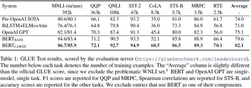
The fine-tuning procedure for GLUE is minimal: batch size 32, 3 epochs, learning rate selected from {5e-5, 4e-5, 3e-5, 2e-5}. The only BERT-specific parameter added is the classification layer — a single weight matrix. The fact that this produces SOTA across nine heterogeneous tasks simultaneously demonstrates that the pre-trained representations are genuinely general-purpose.
SQuAD v1.1 and v2.0
SQuAD v1.1 contains 100,000+ question-passage pairs where the answer is guaranteed to be a span of text within the passage. BERT achieves 93.2 F1 on the test set — exceeding the best ensemble systems of the time using a single model.
SQuAD v2.0 adds unanswerable questions. A model must determine not only where the answer span is, but whether the passage even contains an answer. BERT handles this by treating the [CLS] position as the “null span” — if the no-answer score exceeds the best span score by a learned threshold τ, the model returns no answer. BERT achieves 83.1 F1 on SQuAD v2.0, a 5.1-point improvement over the prior state of the art.
Named Entity Recognition
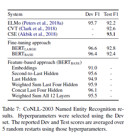
For NER, each token’s final hidden state is passed through a linear layer and softmax to predict an entity label. BERT achieves 92.8 F1 on CoNLL-2003, matching or exceeding prior state-of-the-art systems without any task-specific architectural additions.
Ablation Studies
The ablation studies in Section 5 are the most intellectually valuable part of the paper — they isolate exactly which components of BERT’s design are responsible for its performance.
Effect of Pre-Training Tasks
Four variants were compared:
| Model | What it removes | Key finding |
|---|---|---|
| BERT Base | Nothing (full model) | Baseline |
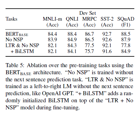
| No NSP | Next Sentence Prediction | Hurts cross-sentence tasks (QNLI −3.5, SQuAD −0.6) |
| LTR & No NSP | Both NSP and bidirectionality | Catastrophic for token tasks (SQuAD −10.7) |
| LTR + BiLSTM | Same, but adds BiLSTM on top | Partially recovers SQuAD, hurts GLUE |
The LTR result is the most important. On SQuAD v1.1, removing bidirectionality drops F1 by 10.7 points. The reason is intuitive: in SQuAD, the question appears before the passage in the concatenated input. A left-to-right model processes the passage without having seen the question yet — it cannot attend to what it needs to find. Bidirectionality allows every passage token to attend to every question token in the same forward pass, which is necessary for span selection.
The BiLSTM result reveals a subtle point: adding a bidirectional post-hoc recurrent layer on top of a left-to-right Transformer partially recovers token-task performance (SQuAD F1 goes from 77.8 to 84.9) but never reaches the full bidirectional baseline (88.5). More importantly, the randomly-initialized BiLSTM hurts GLUE performance — the task-specific recurrent layer degrades the fine-tuned representations for classification tasks. Bolting on bidirectionality at fine-tune time is not equivalent to training bidirectionally from the beginning.
Effect of Model Size
Every increase in L (layers), H (hidden size), or A (attention heads) improves performance monotonically. There are no diminishing returns at the scales tested. This stands in contrast to earlier ELMo work, where increasing hidden size past 1000 showed no benefit.
The reason BERT scales where ELMo does not is the pre-training paradigm. When fine-tuning, only a tiny task-specific head (a few random parameters) is added on top of a large pre-trained model. The task-specific component does not need to “carry” the learning — it redirects rich pre-existing representations. With feature-based methods like ELMo, a larger frozen model gave more features but the same downstream model had to learn from scratch, limiting the benefit.
Feature-Based vs Fine-Tuning
Section 5.3 directly compares the two paradigms for BERT on NER. Even when BERT parameters are frozen and the representations are used only as features for an external model, the results are competitive with fine-tuning:
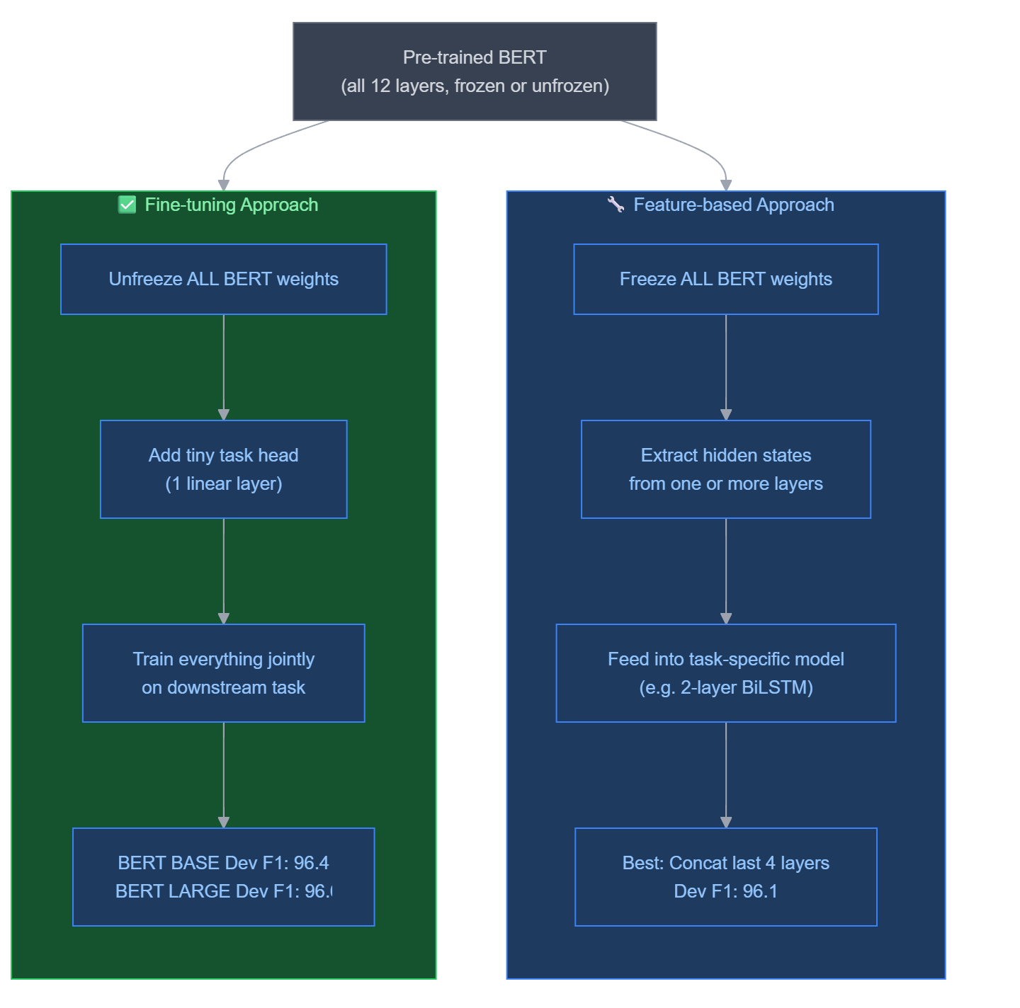
The best feature-based approach — concatenating the top four encoder layers — achieves 96.1 F1, just 0.3 points below the fine-tuned model (96.4 F1). This matters in production: if you cannot afford to fine-tune BERT for every task (due to memory or inference constraints), you can still get near-SOTA performance by treating it as a static feature extractor.
My Understanding
What Actually Makes BERT Work
Reading BERT carefully, the performance gains come from two genuinely different sources that the paper somewhat conflates.
Source 1: Bidirectionality. This is the headline contribution. The ablation studies make it unambiguous — removing bidirectionality costs 10+ F1 points on SQuAD. This is a real architectural advantage, not a training trick. It comes from the fact that BERT uses a Transformer encoder with no causal masking, allowing every token to attend to every other token. The MLM objective is what enables you to train this architecture on a prediction task without the model simply copying the targets.
Source 2: Scale of pre-training. BERT was trained on 3.3 billion words. This is significantly more data than ELMo (800M words from BooksCorpus only) and OpenAI GPT (800M words). It is hard to isolate how much of BERT’s improvement over GPT comes from bidirectionality versus data scale. RoBERTa (2019) addressed this directly: with more data, longer training, and larger batches — but no architectural changes to BERT — performance improved substantially. The conclusion from RoBERTa is that BERT was undertrained. The representations were good, but they could be made significantly better with more compute, without changing anything about the model.
The NSP Question
NSP is the most critiqued part of BERT. The idea is sound — cross-sentence understanding is important for QA and NLI — but the implementation is too easy. Random sentences from the corpus are trivially distinguishable from coherent continuations: they have different topics, different entities, different writing styles. A model could learn to identify NotNext pairs by detecting topic mismatch alone, without learning anything about discourse coherence.
RoBERTa removed NSP entirely and achieved better results. XLNet argued that NSP introduces noise by exposing the model to incoherent inputs that do not appear in natural language. ALBERT replaced NSP with Sentence Order Prediction (SOP) — where both sentences are adjacent but the order is swapped — which is a strictly harder task that requires understanding discourse order rather than just topic overlap.
My read: NSP helps when it helps (multi-sentence tasks like QA and NLI show gains in BERT’s ablations), but it is a weak training signal that is dominated by the MLM contribution. Later work correctly identified and replaced it with a stronger alternative.
What BERT Cannot Do
BERT’s encoder architecture makes it excellent at understanding tasks but fundamentally limited for generation. To generate text autoregressively, you need to produce tokens one by one, conditioning each on the previous ones. But BERT’s bidirectional attention means every position attends to every other position — during generation, the future positions do not exist yet, so you cannot attend to them. You cannot simply run BERT autoregressively.
This is why GPT-style models (decoder-only, causal attention) dominate in text generation, and why sequence-to-sequence tasks (translation, summarisation) require either an encoder-decoder model (T5, BART) or a pure decoder (GPT). BERT’s architecture is fundamentally an understanding architecture.
The Pre-Training Paradigm Shift
The deepest insight from BERT is not any specific architectural choice. It is the demonstration that pre-training quality is the dominant factor in NLP performance, and that sufficiently powerful pre-trained representations transfer to virtually any task with minimal task-specific engineering.
Before BERT, the implicit assumption was that different NLP tasks were fundamentally different problems requiring fundamentally different architectures — parsers for syntactic tasks, attention mechanisms for QA, sequence labellers for NER. BERT showed that all of these tasks share a common bottleneck: the quality of contextual language representations. Solve that bottleneck once at pre-training time, and the task-specific engineering becomes trivial.
This is the shift that opened the path to GPT-3 (175B parameters, zero-shot task performance), to instruction tuning (FLAN, InstructGPT), and ultimately to the large language model paradigm that dominates the field today. BERT was not just a model — it was a proof-of-concept for a research program.
What Came After and Why
| Model | Year | What changed | Why |
|---|---|---|---|
| RoBERTa | 2019 | More data, longer training, no NSP, larger batches | BERT was undertrained; the architecture was not the ceiling |
| ALBERT | 2019 | Parameter sharing + SOP task | Reduce model size while maintaining BERT-level performance |
| XLNet | 2019 | Permutation-based LM (bidirectional without masking) | Avoids the pretrain/finetune mismatch introduced by [MASK] |
| DistilBERT | 2019 | Knowledge distillation from BERT | Efficient BERT for inference-constrained settings |
| T5 | 2019 | Encoder-decoder, frame all tasks as text-to-text | Unify classification and generation under one framework |
| GPT-3 | 2020 | Massive scale decoder, few-shot prompting | Language models are few-shot learners at sufficient scale |
The common thread: every successor either fixed a known BERT limitation (masking mismatch, inefficiency, NSP weakness) or extended the paradigm to cover generation tasks BERT could not handle. None abandoned the core insight — pre-train on massive unlabelled data, then adapt to tasks.
Key Takeaways
-
Bidirectionality is not cosmetic. The ablation studies prove it: removing bidirectionality costs over 10 F1 points on SQuAD. The entire MLM design exists to enable bidirectional training, and it delivers.
-
MLM’s masking strategy is carefully engineered. The 80-10-10 rule prevents the model from ignoring non-masked tokens. The detail matters — a naive 100% masking approach would create a distribution mismatch that degrades fine-tuning performance.
-
NSP is the weak link. It helps cross-sentence tasks modestly but is too easy to drive deep cross-sentence understanding. Subsequent work replaced or removed it. Know when to distrust a sub-component’s contribution claims.
-
Scale unlocks the paradigm. BERT itself was undertrained. RoBERTa showed that more data and longer training with the same architecture substantially improved performance. The architecture is the prerequisite; the training compute is the multiplier.
-
The pre-training paradigm is the real contribution. Not bidirectionality per se, not MLM per se — the proof that a single pre-trained model, fine-tuned with one linear layer, achieves state-of-the-art on eleven diverse tasks simultaneously. That proof changed what researchers tried next.
-
Feature-based and fine-tuning both work. If you cannot fine-tune due to resource constraints, concatenating BERT’s top four layers as static features costs only 0.3 F1 on NER. The representations are good enough to be used either way.
Related Topics
- Attention Is All You Need — the Transformer encoder BERT is built on
- RoBERTa — removes NSP, adds more data, fixes BERT’s undertraining
- XLNet — eliminates the masking mismatch with permutation language modelling
- ALBERT — parameter-efficient BERT with sentence order prediction
- T5 — extends the pre-training paradigm to sequence-to-sequence generation