Why This Paper Matters
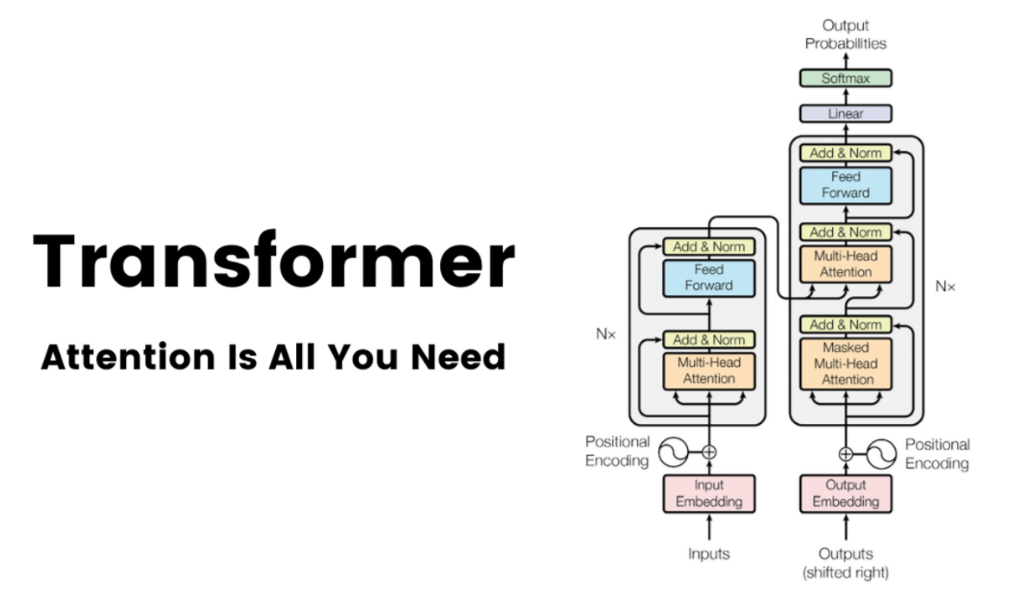
When “Attention Is All You Need” appeared at NeurIPS 2017, it did not merely introduce a faster model. It proposed a fundamentally different answer to the question: how should a model process sequences? The dominant answer for nearly a decade had been recurrence — process tokens one at a time, accumulate a hidden state, let the state carry forward whatever information matters. The Transformer’s answer was: don’t. Route information directly between every pair of positions, in parallel, in a single operation.
To appreciate how radical this was, it helps to understand what the state of the art actually looked like in mid-2017.
The State of the Art Before the Transformer
Sequence-to-sequence models (Sutskever et al., 2014) introduced the encoder–decoder paradigm: an LSTM encoder compresses the source sentence into a fixed-length vector; an LSTM decoder unrolls that vector into the target sequence. The fundamental bottleneck was obvious from the start — compressing an arbitrarily long sentence into a single fixed-size vector loses information, and the decoder had to reconstruct everything from that compressed representation alone.
Bahdanau et al. (2015) introduced neural attention as a remedy. Rather than forcing the encoder to compress everything into one vector, the decoder was allowed to look back at all encoder hidden states and compute a soft weighted average at each decoding step. This was a significant improvement: the “compression bottleneck” was removed, and models could learn to align source words with target words. But crucially, attention here was an add-on mechanism layered on top of recurrent architectures. The RNN was still the backbone; attention was a helpful attachment.
The 2017 paper makes a different claim: attention is not a supplement to recurrent computation — it can replace it entirely. Recurrence is not fundamental to sequence modeling. It is an inductive bias that was useful before modern hardware, but it imposes costs (sequential computation, vanishing gradients, difficulty modeling very long-range dependencies) that outweigh its benefits when the goal is high-capacity, parallelizable training.
Calibrating the BLEU Results
The paper evaluates machine translation primarily using the BLEU (Bilingual Evaluation Understudy) score, a standard benchmark that measures overlap between a candidate translation and one or more human reference translations via n-gram matching (with a brevity penalty).
On the WMT 2014 English→German dataset, the “big” Transformer reported 28.4 BLEU, exceeding previously reported best results — including ensembles — by more than 2 BLEU. To calibrate that number: changing a major design choice like collapsing to a single attention head only reduces BLEU by roughly 1 point. So a +2 point improvement is unusually large. In competitive MT benchmarks, even ~1 BLEU can be meaningful. A +2 shift is typically interpreted as a qualitative architectural leap, not a minor tweak.
On English→French, the big model achieved 41.0 BLEU, a new state-of-the-art trained in less than a quarter of the time of previous best models. This cost argument is just as important as the accuracy argument — it tells us that the architecture scales better and that more compute translates into more performance more predictably.
The Downstream Cascade
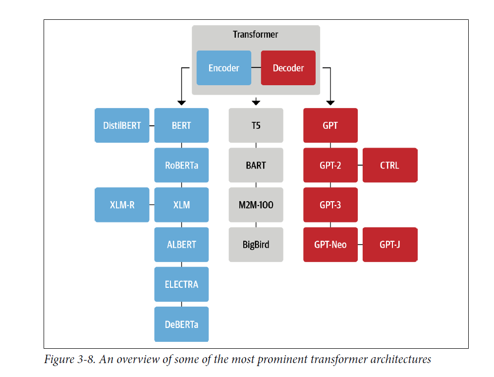
The Transformer was not just the best model of 2017. It became the substrate for essentially every important language model that followed. BERT (2018) uses the encoder. GPT (2018) uses the decoder. T5 (2019) uses the full encoder-decoder. GPT-3 (2020), PaLM (2022), LLaMA (2023), and every frontier LLM through 2025 are Transformer decoders at their core. The architecture generalised far beyond machine translation to code generation, reasoning, image captioning, protein structure prediction, and reinforcement learning. Understanding this paper is not optional background — it is the bedrock of contemporary AI.
The Pre-Transformer Landscape: Why Recurrence and Convolution Were Limiting
Before Transformers, the dominant approaches to sequence transduction were:
- Recurrent models (RNNs, LSTMs, GRUs)
- Convolutional sequence models (ByteNet, ConvS2S)
Each family has a characteristic failure mode. Understanding both is necessary to appreciate why the Transformer’s design choices are not arbitrary — they are precise engineering responses to specific, measurable problems.
The Fundamental Constraint of Recurrent Computation
Recurrent models factor computation over time steps. At step t, the hidden state depends on the previous step. This enforces sequential computation within each example, which limits parallelization. As sequence length grows, it becomes harder to batch effectively (memory constraints), and training time increases. Long-range dependencies become harder because the computational path between distant tokens grows with distance.
More precisely, the maximum path length between any two positions in a recurrent model is O(n) — to pass information from the first token to the last token in a length-n sequence, you must traverse every intermediate hidden state. This path length is directly related to how hard it is to learn long-range dependencies: the longer the path, the more operations a gradient must travel through during backpropagation, and the more likely it is to vanish or explode.
The vanishing gradient problem in RNNs is not merely a theoretical concern. In practice, unmodified RNNs struggle to capture dependencies spanning more than 10–20 tokens. LSTMs and GRUs were specifically designed to address this by gating information flow — but they do not eliminate the O(n) path length. They make the path traversable for moderate lengths, not short.
Simple RNN: Minimal Recurrence
h_t = σ(W_h · h_{t-1} + W_x · x_t + b)
The simplest formulation: the hidden state is a function of the previous hidden state and the current input. Expressive in principle, but the sequential dependency is a hard constraint. Gradients must flow through the same weight matrix W_h at every time step, which causes exponential decay (vanishing) or exponential growth (exploding) over long sequences.
LSTM: Gated Memory via Cell State
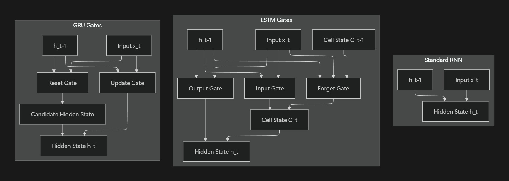
LSTMs add a persistent memory cell (C_t) and three gates — forget, input, and output — to control information flow:
f_t  = σ(W_f [h_{t-1}, x_t] + b_f)        # forget gate
i_t  = σ(W_i [h_{t-1}, x_t] + b_i)        # input gate
C̃_t = tanh(W_C [h_{t-1}, x_t] + b_C)     # candidate cell
C_t  = f_t ⊙ C_{t-1} + i_t ⊙ C̃_t         # cell state update

o_t  = σ(W_o [h_{t-1}, x_t] + b_o)        # output gate
h_t  = o_t ⊙ tanh(C_t)                    # hidden state
The cell state C_t is the key innovation: it is updated by addition (not multiplication through a squashing function at every step), so gradients can flow along the cell state pathway with much less attenuation. The forget gate provides a learnable mechanism for the model to decide which information to preserve and which to discard. The cell state provides a highway for gradients, which helps with longer dependencies — but the sequential bottleneck remains. You still cannot compute ht until you have h{t-1}.
GRU: Simplified Gating
GRUs streamline the gating mechanism into two gates (reset and update), while preserving the same sequential dependency:
z_t  = σ(W_z [h_{t-1}, x_t] + b_z)        # update gate
r_t  = σ(W_r [h_{t-1}, x_t] + b_r)        # reset gate
h̃_t = tanh(W [r_t ⊙ h_{t-1}, x_t] + b)   # candidate hidden state
h_t  = (1 - z_t) ⊙ h_{t-1} + z_t ⊙ h̃_t   # hidden state
The input and previous hidden state feed into the reset gate and update gate. The reset gate modulates how much of the past hidden state enters the candidate, and the update gate interpolates between old and new. GRUs have fewer parameters than LSTMs (no output gate, no separate cell state) and are computationally cheaper per step while achieving comparable performance on many tasks. But the sequential dependency is identical — GRUs did not solve the parallelization problem.
Convolutional Models and the Long-Distance Problem
Convolutional approaches like ByteNet (Kalchbrenner et al., 2016) and ConvS2S (Gehring et al., 2017) attacked the parallelization problem directly. By replacing recurrence with 1D convolutions over sequence positions, they enabled parallel computation within each layer — the operation at position i does not depend on the operation at position i-1 within the same layer.
This was a genuine improvement. ConvS2S achieved strong MT results and trained significantly faster than LSTMs. But it introduced a different problem: the receptive field grows only as fast as network depth. A kernel of width k can only “see” k adjacent positions in a single layer. To connect tokens that are far apart, you need many layers — the maximum path length between two positions scales as O(log_k(n)), which is better than O(n) but still grows with sequence length.
For very long sequences, this means either building very deep networks or accepting that distant tokens cannot directly interact. The Transformer’s self-attention reduces this path length to O(1): any token can attend to any other token in a single attention operation, regardless of how far apart they are.
Parallelism alone is not enough. Models must also allow direct interaction between arbitrary positions without requiring many layers of intermediate computation.
Mental model:
- RNNs are a word-by-word reader: expressive but inherently sequential, O(n) path length.
- CNNs are a parallel scanner: fast but need depth to connect far-apart positions, O(log n) path length.
- Transformers are a parallel matchmaker: every position talks to every other position directly, O(1) path length.
The Transformer’s Central Idea
The Transformer proposes a model that removes recurrence and convolution entirely, using attention as the only sequence interaction mechanism, with pointwise MLPs for per-token processing. This enables high parallelization during training.
Two linked motivations:
- Optimization / Engineering: Break the sequential computation bottleneck to maximize parallelism on modern hardware.
- Representation: Allow every token to directly condition on every other token, making long-range dependencies easier to learn.
The conceptual shift is not merely that “attention helps,” but that sequence modeling can be built entirely from global, content-based routing (attention) plus local non-linear transformation (position-wise FFN).
The Design Philosophy
Every design choice in the Transformer follows from a clean decomposition of what sequence modeling actually requires:
-
Tokens need to exchange information — attention handles this. It is a learned, content-based routing system: each token broadcasts a query describing what it’s looking for, and all other tokens broadcast keys describing what they offer. Compatibility scores determine how much information flows.
-
Each token needs to process its own representation — the position-wise FFN handles this. After information has been routed via attention, each token independently transforms its updated representation through a small two-layer MLP.
-
Deep models need stable training — residual connections and layer normalisation handle this. They prevent representational collapse and allow gradients to flow reliably through many layers.
-
Sequences have order — positional encodings handle this. Without them, attention is permutation-invariant, meaning the model would produce the same output regardless of token order.
This separation of concerns is elegant: interaction is handled by attention, transformation is handled by FFN, stability is handled by normalisation, and order is handled by encoding. Nothing is conflated.
Attention as a Computation Primitive
An attention function maps a query and a set of key–value pairs to an output vector. The output is a weighted sum of values, where the weight for each value is determined by the compatibility of the query with the corresponding key.
Query / Key / Value Roles
The same input representation is projected into three distinct roles:
- Query (Q): What this position is looking for.
- Key (K): What this position offers — how it should be matched against.
- Value (V): The information to be aggregated if matched.
Self-attention is a learned weighted averaging mechanism over token representations. The weights come from comparing queries to keys; the content that flows comes from the values.
Given input matrix X (shape: sequence length n × model dimension d_model), the projections are linear:
Q = X · W_Q     # shape: n × d_k
K = X · W_K     # shape: n × d_k
V = X · W_V     # shape: n × d_v
The projection matrices WQ, W_K, W_V are learned parameters. The fact that Q, K, and V all originate from the same X (in self-attention) does not mean they contain the same information — the learned projections carve out different subspaces. W_Q asks: “what aspects of my current state are useful for _finding information?” WK asks: “what aspects of my state are useful for _being found?” WV asks: “what information should I _contribute if found?”
This separation is important. A token can be easy to attend to (high key similarity with many queries) while contributing subtly different information through its value. The decoupling gives the model more representational flexibility than a single projection would.
Scaled Dot-Product Attention: Step by Step
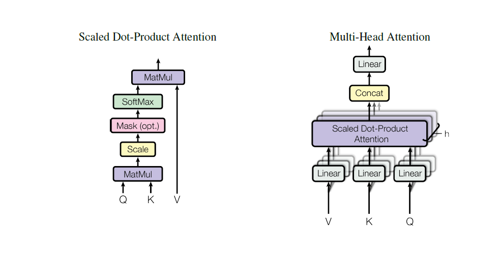
Attention(Q, K, V) = softmax(Q K^T / √d_k) · V
Where d_k is the query/key dimensionality per head and QK^T produces an n × n matrix of pairwise similarity scores.
Let’s walk through this operation concretely for a 4-token sequence (“The”, “cat”, “sat”, “down”):
Step 1 — Compute raw similarity scores: Form the matrix product QK^T (shape: n × n). Entry [i, j] is the dot product of query i with key j — how much token i “wants to attend to” token j. High values mean high affinity.
Step 2 — Scale: Divide every entry by √d_k. This is not optional normalisation — it has a specific purpose described below.
Step 3 — Softmax per row: Apply softmax across each row of the scaled score matrix. Each row now sums to 1 and represents a probability distribution over positions — the attention weights for token i attending over all positions.
Step 4 — Weighted sum of values: Multiply the attention weight matrix (n × n) by V (n × d_v). Each row of the result is a weighted average of value vectors, where the weights came from the similarity computation in steps 1–3.
The output is a new representation for each token — the same shape as the input, but enriched by information drawn from all positions according to learned relevance.
Why the √d_k Scaling Exists
With large d_k, dot products can grow large in magnitude. To see why: if Q and K have entries drawn from a distribution with mean 0 and variance 1, then Q·K (a sum of dk products) has mean 0 but variance d_k. For d_k = 64, the standard deviation of the dot product is √64 = 8. When dot products grow large in magnitude, the softmax function is pushed into regions where its gradient is near zero — essentially, one score dominates and the distribution collapses toward a one-hot vector. This kills learning. Scaling by _1/√d_k brings the variance back to approximately 1 and keeps the softmax in a trainable region.
The paper notes this issue explicitly: for small d_k, additive and dot-product attention perform similarly, but for larger d_k, unscaled dot-product attention underperforms without the scaling fix.
Dot-Product vs. Additive Attention
Two common attention families exist:
- Additive attention (Bahdanau-style): compatibility computed by a small feed-forward network: score(q, k) = v^T · tanh(W_q · q + W_k · k). This adds parameters and is slower.
- Dot-product attention: compatibility computed by inner product: score(q, k) = q · k.
Dot-product attention is faster and more space-efficient in practice thanks to optimized matrix multiplication (BLAS routines, tensor cores on modern GPUs). For large dimensions, additive attention can outperform unscaled dot-product attention because it avoids the saturation problem — the scaling factor is a targeted fix for this at no extra parameter cost.
Multi-Head Attention
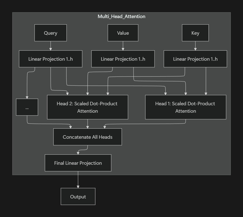
Single-head attention produces one weighted average per token — a single “reading” of the sequence. Multi-head attention runs attention in parallel across multiple learned projection subspaces:
head_i = Attention(Q · W_i^Q,  K · W_i^K,  V · W_i^V)

MultiHead(Q, K, V) = Concat(head_1, ..., head_h) · W^O
The paper uses h = 8 heads. With d_model = 512, each head operates in a d_k = d_v = 512/8 = 64-dimensional subspace. The total parameter count is the same as single-head attention in a 512-dimensional space — multi-head attention is not more expensive in terms of parameters, but it extracts far richer structure from the same computational budget.
What Multi-Head Attention Buys You
A single attention head produces one weighted average, which can behave like an averaging blur — the model cannot simultaneously focus sharply on a syntactic dependency and a semantic association from the same representation. Multiple heads mitigate this by letting the model attend to different representation subspaces simultaneously.
Consider the sentence: “The Law will never be perfect, but its application should be just.” Different heads can specialise in different phenomena:
- One head resolves “its” → “The Law” (anaphora / coreference): high attention weight from “its” to “Law”.
- Another aligns “its” with “application” for local syntactic structure: high attention weight from “its” to “application”.
- A third might track the discourse structure, marking the contrast introduced by “but”.
Mental model: Multi-head attention is a committee of specialist readers. Each reads for a different phenomenon — syntax, semantics, coreference, discourse — then the model combines their evidence via the output projection W^O.
The Output Projection W^O
After concatenating all h head outputs (giving a vector of size h × d_v = d_model), the output projection W^O (shape: d_model × d_model) mixes information across heads. This is essential: individual heads encode information in disjoint subspaces; the output projection re-integrates those subspaces into a single coherent representation for the next layer.
Self-Attention: What It Replaces and Why
Self-attention relates positions within a single sequence. In self-attention, Q, K, and V all come from the same sequence (in contrast to cross-attention, where Q comes from the decoder and K, V come from the encoder).
Core Motivations
- Constant path length: Any token can directly attend to any other token in a single attention step, easing long-range dependency learning. This is the O(1) path length advantage over RNNs (O(n)) and CNNs (O(log n)).
- Parallelism: Removes the sequential bottleneck of recurrence. All positions are processed simultaneously within a layer.
- Interpretability: Attention maps can sometimes be inspected to reveal learned linguistic structures (coreference, syntactic dependencies). This is not guaranteed — attention weights are not the same as “what the model used” — but it provides more introspective access than recurrent hidden states.
Each token representation becomes a context-dependent mixture of other token value vectors. Ambiguity resolution emerges naturally because different contexts induce different attention patterns.
The Complexity Trade-Off Table
The paper includes an explicit comparison of computational properties across model types. This is one of the most practically important tables in the paper and is worth reproducing carefully:
| Layer Type | Complexity per Layer | Sequential Operations | Max Path Length |
|---|---|---|---|
| Self-Attention | O(n² · d) | O(1) | O(1) |
| Recurrent (RNN/LSTM) | O(n · d²) | O(n) | O(n) |
| Convolutional (kernel k) | O(k · n · d²) | O(1) | O(log_k(n)) |
| Self-Attention (restricted r) | O(r · n · d) | O(1) | O(n/r) |
Where n = sequence length, d = model dimension, k = kernel size, r = neighborhood size for restricted attention.
Key observations from this table:
- Self-attention has O(1) sequential operations — no step depends on a previous step, so the entire layer runs in parallel.
- Self-attention has O(1) max path length — any two positions interact directly, no matter how far apart.
- Self-attention has O(n²·d) complexity — this is the cost. For translation-length sequences (n ≈ 100), this is fine. For document-length contexts (n ≈ 10,000+), the n² term becomes prohibitive — motivating later efficiency work (Longformer, BigBird, FlashAttention).
- Recurrent has O(n) sequential operations — this is the fundamental bottleneck. No matter how fast each step is, you cannot process step t until step t-1 is done.
When n < d (common at translation-length sequences), self-attention is also faster in practice than recurrence. The paper explicitly notes this: the key practical win for typical NLP sequence lengths is that O(n²·d) beats O(n·d²) when n ≪ d.
The Trade-Off: Quadratic Cost
Self-attention forms an n × n attention matrix per head per layer. For a model with 6 layers, 8 heads, and d_k = 64, processing a sequence of length 100 requires storing attention matrices totaling 6 × 8 × 100 × 100 = 4.8M floating point values. For n = 1,000, this becomes 480M values — already heavy. For n = 10,000, it becomes 48B values — intractable without approximations.
This quadratic scaling in context length was the primary limitation that subsequent work (Sparse Transformers, Reformer, Longformer, FlashAttention) addressed. But for the original paper’s use case — sentence-level machine translation — it was entirely acceptable.
Key distinction:
- Self-attention primarily addresses the sequence-length interaction problem: how do we let distant tokens communicate without long sequential paths?
- Residual connections + normalization primarily address the depth / optimization problem: how do we train networks with many layers without gradient vanishing or representational collapse?
Position-Wise Feed-Forward Networks
Each encoder/decoder layer contains a position-wise FFN applied independently and identically at each position:
FFN(x) = max(0, x · W_1 + b_1) · W_2 + b_2
“Position-wise” means the same FFN parameters are applied to every token position. There is no cross-token mixing in the FFN; cross-token mixing happens exclusively in attention. While input and output stay at d_model (512), the inner FFN dimension is much larger (d_ff = 2048 in the base model), providing additional capacity via an expand-then-contract bottleneck.
Why the Expansion-Contraction Pattern?
The ratio d_ff / d_model = 2048 / 512 = 4 is a deliberate design choice. The expansion to 2048 dimensions gives each token access to a high-dimensional processing space where complex, non-linear transformations can occur. The subsequent contraction back to 512 forces the model to compress that processing into the representational bottleneck.
This pattern has an interesting interpretation: the expanded layer can be seen as a key-value memory (Geva et al., 2021 showed this empirically). Each row of W_1 acts as a “key” that fires for specific input patterns, and the corresponding column of W_2 is the “value” that contributes to the output. The model stores factual associations and linguistic transformations in these weight matrices.
The Role of ReLU
The ReLU activation max(0, ·) is applied element-wise after the first linear transformation. This introduces sparsity — many neurons in the expanded layer fire at zero — and non-linearity. Without non-linearity, the two-layer FFN would collapse to a single linear transformation and provide no additional capacity over a single matrix multiplication.
Mental model: Attention is communication between positions — it determines what information flows where. The FFN is per-token computation — it processes each token’s updated representation independently, applying learned transformations that do not depend on what other tokens are doing.
Positional Encoding: Injecting Order
Attention is permutation-invariant unless we inject order. If you shuffle all tokens in the input and apply attention with the same weights, you get the same output vectors (just shuffled). The Transformer cannot distinguish “The cat sat” from “sat cat The” without some positional signal. Positional encoding solves this by adding order information directly to the embeddings before any processing.
Operational order: Token IDs → embedding lookup → add positional encoding → first Transformer layer.
The positional encoding has the same dimension as the model (d_model = 512), so it can be added element-wise to the token embedding.
Sinusoidal Positional Encoding (Original Paper)
PE(pos, 2i)   = sin(pos / 10000^(2i / d_model))
PE(pos, 2i+1) = cos(pos / 10000^(2i / d_model))
Each position gets a unique vector of sin/cos values at different frequencies. The wavelengths form a geometric progression from 2π (for the highest-frequency dimension, 2i = 0) to 20000π (for the lowest-frequency dimension, 2i = d_model - 2).
Why Sinusoidal?
The sinusoidal choice has two important properties that the authors highlight:
Unique per position. No two positions produce the same encoding vector, so the model can distinguish every position.
Relative offset linearity. For any fixed offset k, PE(pos + k) can be expressed as a linear function of PE(pos). This means the model can in principle learn to attend by relative position — “two tokens ahead” — by learning the appropriate linear transformation, without needing to hard-code absolute positions.
Concretely: sin(pos + k) = sin(pos)cos(k) + cos(pos)sin(k). The sin and cos components of position pos can be linearly combined to produce the encoding at position pos + k, with coefficients that depend only on k, not pos.
Potential extrapolation. Sinusoidal encodings can be generated for any position, including positions longer than any sequence seen during training. Learned positional embeddings cannot generalize to positions not seen during training — they have no defined value for those positions.
Key insight: Positional encoding provides coordinates — it tells the model where each token is. Attention provides relational meaning — it determines what information flows based on content. These two mechanisms compose: the model can learn to attend to specific positions and to specific content simultaneously, because the positional signal is baked into the representation before attention is computed.
The Transformer Architecture
High-Level Roles
- Encoder: Produces contextualised representations of the input (often called “memory”). Every token in the encoder representation can attend to every other token — there is no masking.
- Decoder: Generates output autoregressively while attending to both past output tokens (masked self-attention) and encoder memory (cross-attention). The decoder cannot attend to future positions in its own sequence (they haven’t been generated yet).
Residual Connections and Layer Normalization
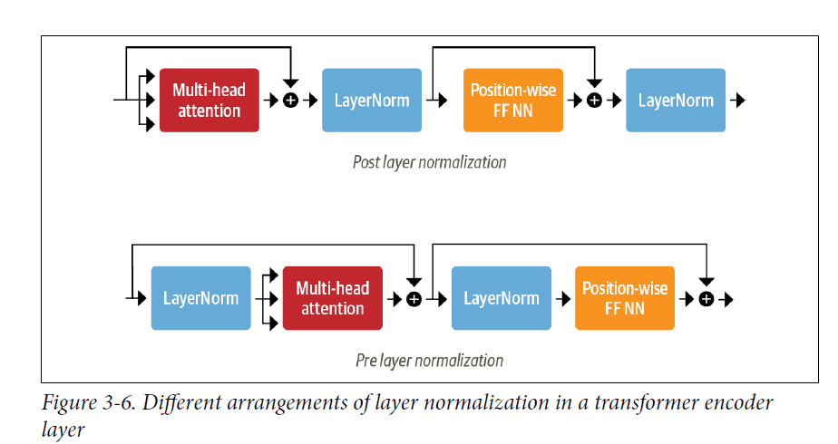
The original paper uses the Post-LN pattern:
LayerNorm(x + Sublayer(x))
This wraps every sublayer (multi-head attention or FFN) in a residual connection followed by layer normalisation.
Why residual connections are essential at scale: In a deep network, the forward pass is a composition of many functions. Without residual connections, each layer must learn a full transformation — small errors compound multiplicatively. With residual connections, each layer learns a correction to its input rather than a full transformation. During backpropagation, gradients can flow directly through the identity path (the shortcut) without passing through any non-linearities, providing stable gradient signals to early layers even in 6-layer or 12-layer networks. This is the same idea that made ResNet transformative for computer vision (He et al., 2016).
Why layer normalisation works here: Unlike batch normalisation (which normalises across the batch dimension), layer normalisation normalises each sample independently across its feature dimension. This makes it suitable for variable-length sequences where batch statistics would be unstable. It stabilises the scale of activations entering each sublayer, which is especially important when residual additions can cause activation magnitudes to grow across layers.
Post-LN vs Pre-LN: The original Transformer applies normalisation after the residual addition. A common modern variant (Pre-LN, used in GPT-2 and most subsequent work) applies normalisation before the sublayer. Pre-LN is generally more stable during training and does not require the careful learning-rate warmup that Post-LN does — it allows larger learning rates and more aggressive training schedules. Most current LLMs use Pre-LN.
The Encoder
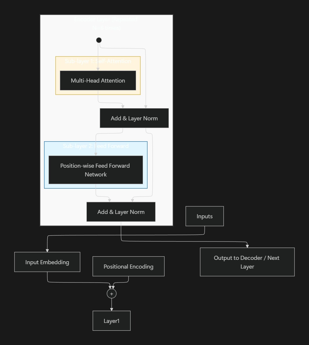
The encoder consists of a stack of N = 6 identical layers. Each layer has two sublayers:
- Multi-head self-attention: All tokens attend to all tokens. Every token can incorporate information from every other token in a single layer.
- Position-wise FFN: Each token independently processes its updated representation.
Both sublayers are wrapped in residual + layer norm. The output of each encoder layer is a set of n vectors of dimension d_model — one per input token — where each vector encodes that token in the context of all other tokens.
After N = 6 layers, the encoder produces its final output: a sequence of context-rich vectors that the decoder will use via cross-attention.
The Decoder
The decoder also consists of N = 6 identical layers. Each decoder layer has three sublayers:
- Masked multi-head self-attention — prevents “peeking” at future tokens. The decoder attends only to already-generated positions in its own output.
- Encoder–decoder attention (cross-attention) — queries come from the decoder’s current state, keys and values come from the encoder’s final output (memory). This is the mechanism that connects the source sentence to the generation process.
- Position-wise FFN — same as the encoder.
All three sublayers are wrapped in residual + layer norm.
Why Masking Is Required
To preserve autoregressive generation, token at position i must not depend on tokens at positions j > i. If masking were absent, during training the decoder could look ahead at future tokens, trivially copy them, and achieve perfect training loss without learning anything useful — the learned function would not generalize to inference where future tokens are unavailable.
Implementation: set illegal attention logits (those corresponding to future positions) to −∞ before softmax. exp(−∞) = 0, so those positions receive exactly zero weight after softmax, effectively blocking information flow from future positions.
Cross-Attention: The Bridge Between Encoder and Decoder
Cross-attention is where the decoder “reads” the source sentence. It is structurally identical to self-attention except that Q is computed from the decoder’s current states and K, V are computed from the encoder’s final output. This means:
- The decoder’s current state (what has been generated so far) forms the query: “given what I’ve written, what in the source should I focus on next?”
- The encoder memory provides the keys and values: “here is everything the encoder has learned about the source.”
This is the learned alignment mechanism that replaced the Bahdanau attention of earlier seq2seq models — but now operating over rich, contextualised representations produced by 6 layers of self-attention, not over raw LSTM hidden states.
Decoder Step-by-Step
- Input tokens (generated-so-far in inference; shifted targets in training) are embedded and combined with positional signals.
- Masked self-attention uses only left context — each generated token attends to all previously generated tokens.
- Cross-attention queries the encoder memory — each decoder state forms a query over all encoder positions.
- Output projection + softmax produces a probability distribution over the vocabulary for the next token.
Training vs. Inference
Training (Teacher Forcing + Masking)
Transformers preserve autoregressive constraints while enabling parallel training — this is a crucial practical advantage over RNNs at training time.
- The encoder processes the entire source sentence at once, in parallel.
- Decoder input is the target sequence shifted right by one position (starts with
<Start>, ends with the last real token). - The causal mask ensures token at position i cannot attend to positions > i.
- The model predicts the probability distribution for each target token simultaneously — all positions in parallel.
- Loss is the cross-entropy between predicted distributions and ground-truth tokens, summed over positions.
- Gradients backpropagate through all layers simultaneously.
This teacher forcing approach — using ground-truth previous tokens as decoder inputs at each training step — is what enables parallel training. At training time, we always know the entire target sequence, so we can feed the entire shifted target as input and compute all output distributions in one forward pass.
Inference (Autoregressive Loop)
- Encoder processes the input once and caches its output (encoder memory does not change during decoding).
- Decoder starts from
<Start>and generates one token at a time. - Each newly predicted token is appended to the decoder input sequence.
- At each step, the decoder reprocesses the growing sequence (though the encoder output is fixed).
- Generation stops when the model produces
<EOS>or a maximum length is reached.
Key insight: Training is fully parallel; inference is sequential. This creates the exposure bias problem: at training time, the model sees correct previous tokens (teacher forcing), but at inference time it sees its own (potentially erroneous) previous outputs. Errors at early positions can cascade. This is a known limitation of the teacher forcing paradigm and has motivated research into curriculum learning, scheduled sampling, and non-autoregressive decoding.
Training Regime and Engineering Details
Understanding the training setup is important because many design choices that appear arbitrary are actually tightly coupled to the loss landscape of deep attention networks.
Datasets: WMT 2014 English–German (~4.5M sentence pairs, BPE-encoded with a shared vocabulary of ~37k tokens) and English–French (36M sentence pairs, word-piece vocabulary of ~32k tokens). Byte-pair encoding (BPE) is crucial: it produces a vocabulary of subword units that balances coverage of rare words (which character-level models handle but word-level models cannot) with vocabulary size efficiency.
Batching: Batches are grouped by approximate sequence length, each containing ~25k source tokens and ~25k target tokens. This length-based batching reduces padding waste and improves hardware utilization significantly.
Hardware: A single machine with 8 NVIDIA P100 GPUs. The base model (d_model = 512, 65M parameters) was trained for 100k steps in approximately 12 hours. The big model (d_model = 1024, 213M parameters) was trained for 300k steps in approximately 3.5 days.
The Learning Rate Schedule
Optimization: Adam with β₁ = 0.9, β₂ = 0.98, ε = 10⁻⁹. The learning rate follows a specific schedule:
lrate = d_model^(-0.5) · min(step_num^(-0.5), step_num · warmup_steps^(-1.5))
This schedule increases the learning rate linearly for the first warmup_steps = 4000 steps, then decreases it proportionally to the inverse square root of the step number.
Why warmup? In the early stages of training, the model weights are randomly initialised and the gradient estimates are noisy. A large initial learning rate would cause the model to diverge — especially important for the Post-LN variant used in this paper, where gradients at early layers can be large before the model has begun to learn stable representations. The warmup phase ensures the model first navigates to a reasonable region of parameter space before using the full learning rate.
Why inverse-sqrt decay? As training progresses, finer adjustments are needed. The model has already found a good region of loss landscape and needs to refine rather than explore. The inverse-sqrt schedule provides a principled decay that balances exploration early and exploitation late.
Regularization
Residual dropout (p = 0.1): Applied to the output of each sublayer before it is added to the residual connection, and to the sums of embeddings and positional encodings. Dropout prevents co-adaptation — neurons cannot rely on specific other neurons being active, which forces the model to learn more robust, distributed representations.
Label smoothing (ε = 0.1): Instead of training the model to output probability 1.0 for the correct token and 0.0 for all others, label smoothing targets a distribution where the correct token gets probability (1 − ε) = 0.9 and the remaining ε = 0.1 is distributed uniformly across all other tokens. The paper notes this hurts perplexity (the model can no longer be maximally confident) but improves BLEU and accuracy. This makes sense: over-confident models that assign near-zero probability to all non-target tokens are poorly calibrated and fail to generalise — label smoothing forces the model to maintain non-trivial distributions over alternatives.
Checkpoint averaging: The final model is not taken from the last checkpoint but from an average of the last 5 (base) or 20 (big) checkpoints, saved at 10-minute intervals. Averaging parameters across training checkpoints approximates an ensemble of models at different points in the training trajectory, providing better generalisation at zero additional inference cost.
Ablation Study: What Actually Matters
The paper includes a systematic ablation study on the English→German translation task. This table is one of the most instructive parts of the paper because it isolates the contribution of each design decision.
| Model Variant | EN→DE BLEU | Params |
|---|---|---|
| Base model (h=8, d_k=64, d_ff=2048, P_drop=0.1) | 25.8 | 65M |
| Single head (h=1) | 24.9 (−0.9) | same |
| Too many heads (h=32, d_k=16) | 25.5 (−0.3) | same |
| Reduced d_k (h=16, d_k=32) | 25.5 (−0.3) | same |
| Larger model (d_model=1024) | 26.4 (+0.6) | 213M |
| No dropout | 25.3 (−0.5) | 65M |
| Learned positional embeddings | 25.5 (−0.3) | 65M |
| Big model (2× layers, 2× heads, 2× dims) | 28.4 | 213M |
Key takeaways:
Head count matters, but not linearly. Using only one head loses 0.9 BLEU — significant. But using too many heads (32 with d_k = 16) also slightly underperforms the base 8-head configuration. Each head operates in a very low-dimensional subspace (16 dimensions) and may not have enough capacity to learn a useful specialisation. The sweet spot is moderate head count with sufficient per-head dimension.
Reducing d_k hurts. When d_k drops from 64 to 32 (by doubling heads to 16), performance falls. This supports the hypothesis that per-head capacity is important, and that the dot-product attention mechanism benefits from a minimum dimensionality to form meaningful similarity comparisons.
Dropout is essential. Removing dropout drops 0.5 BLEU. The model overfits without it.
Positional encodings are roughly equivalent. Replacing sinusoidal encodings with learned positional embeddings costs only 0.3 BLEU — a nearly negligible difference. This suggests that the specific choice of positional encoding is less important than simply having some positional signal. Most subsequent work (BERT, GPT) has used learned positional embeddings.
Scale is the dominant factor. The big model (4× more parameters, 3× longer training) delivers the 28.4 BLEU headline number. Architectural improvements provide the foundation; scale provides the ceiling.
Architectural Variants: Encoder-Only, Decoder-Only, Encoder–Decoder
The Transformer was originally designed as a full encoder-decoder for machine translation. But the general architecture proved extraordinarily flexible — its components can be recombined to suit different tasks.
Encoder-Only (BERT-Style): Bidirectional Representations
Encoder-only models compute representations where each token depends on both left and right context — the full sequence is available at every position. Best suited for understanding tasks: classification, named entity recognition, question answering, textual entailment. The training objective is typically masked language modelling (MLM): randomly mask 15% of tokens and train the model to predict them from bidirectional context.
The architectural point is bidirectionality: because every token can attend to every other token with no masking, the representation of “bank” in “the bank of the river” can incorporate “river” even though it appears after “bank.” This full bidirectionality is not possible in decoder-only models.
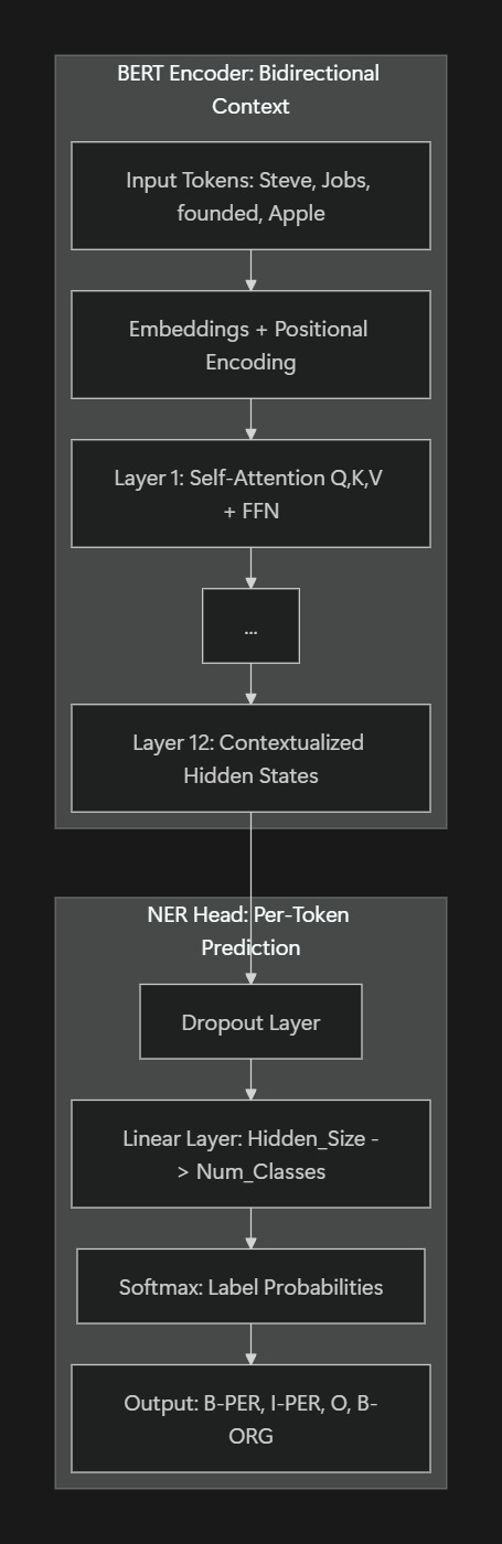
BERT (Devlin et al., 2018) became the dominant pre-training paradigm for NLP understanding tasks through 2019–2021. RoBERTa, ALBERT, DeBERTa, and many domain-specific variants (BioBERT, ClinicalBERT, FinBERT) all use the encoder-only architecture.
Decoder-Only (GPT-Style): Causal Generation
Decoder-only models implement causal masking so each token depends only on its left context. Optimised for next-token prediction and generation. The training objective is language modelling (LM): predict the next token given all previous tokens.
The full Transformer decoder minus the cross-attention sublayer becomes the entire backbone. Without cross-attention, there is no encoder to attend to — the decoder attends only to its own past outputs via masked self-attention.
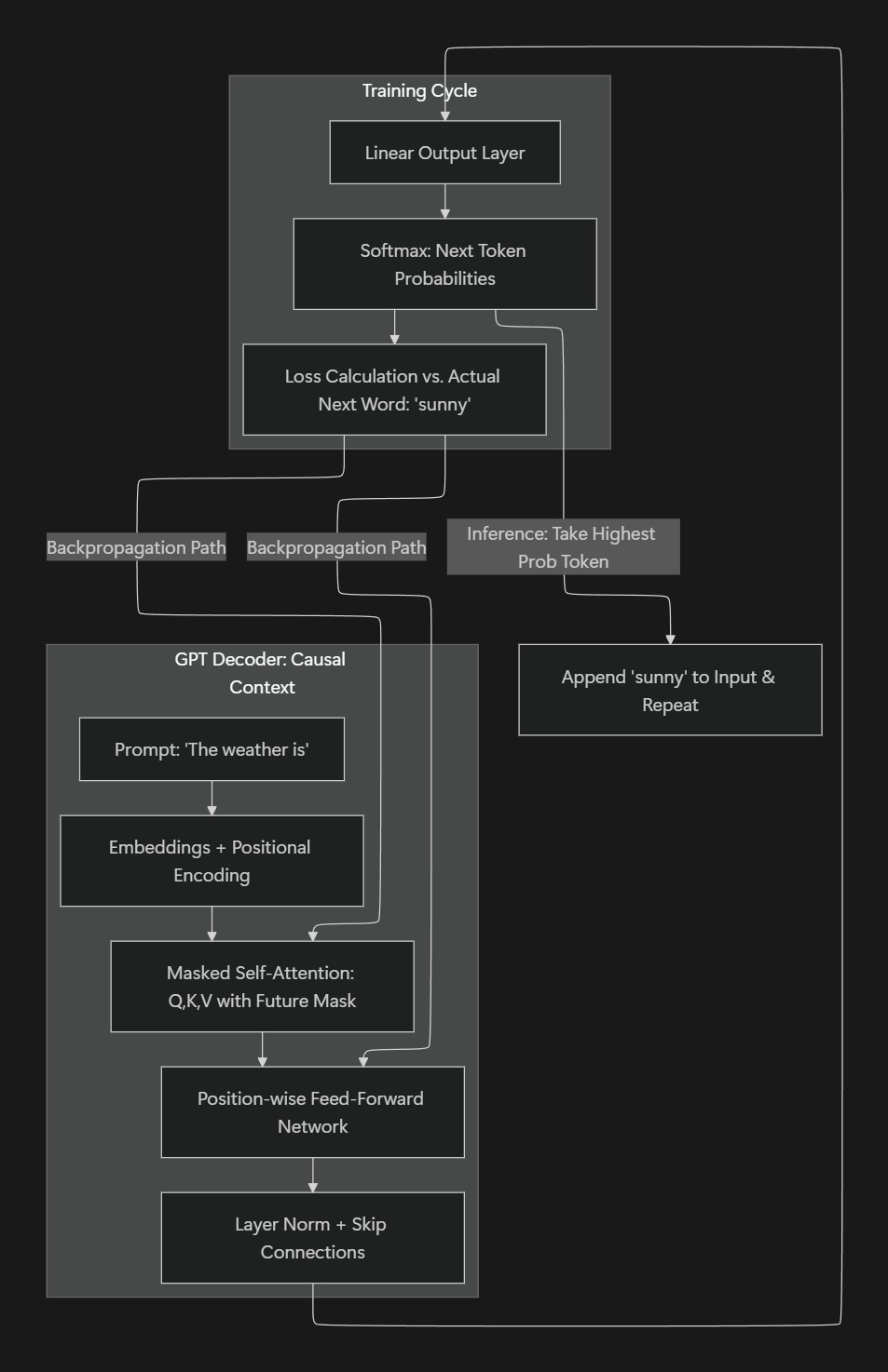
GPT (Radford et al., 2018) introduced this paradigm. GPT-2 (2019) demonstrated that larger decoder-only models can do zero-shot and few-shot task completion without fine-tuning. GPT-3 (2020) scaled this to 175B parameters and demonstrated in-context learning at unprecedented scale. GPT-4, Claude, Gemini, and LLaMA are all decoder-only architectures.
The decoder-only architecture has come to dominate frontier model development because:
- It scales more cleanly than encoder-decoder on a single, unified next-token-prediction objective.
- The same model can do generation, summarisation, translation, and classification without architectural changes — just different prompting.
- KV-cache makes autoregressive inference efficient: encoder representations are cached and reused, eliminating redundant computation on context tokens during generation.
Encoder–Decoder: Sequence-to-Sequence
Encoder–decoder architectures model conditional generation explicitly. The encoder builds a rich contextual representation of the input; the decoder generates the output conditioned on that representation via cross-attention. Tasks that are naturally framed as transformation of one sequence into another — translation, summarisation, question generation, code generation from docstrings — are well-suited to this architecture.
T5 (Raffel et al., 2019) reframed all NLP tasks as seq2seq text generation, using an encoder-decoder Transformer as a unified backbone. BART (Lewis et al., 2020) combined a denoising encoder pre-training objective with an autoregressive decoder for generation, achieving strong performance on summarisation. More recently, encoder-decoder models have been applied to structured prediction, multi-modal generation (image captioning), and speech recognition.
How Embeddings Become Contextual Representations
The central throughline of the Transformer is the journey from static, context-independent token embeddings to rich, context-sensitive representations through repeated self-attention + FFN blocks.
At layer 0, each token is simply its embedding vector — a fixed point in d_model-dimensional space. The word “bank” at layer 0 is the same vector regardless of whether it appears in a financial context or a riverbank context. By layer 6 (in the base model), the representation of “bank” has been enriched by 6 rounds of information exchange with every other token in the sequence. The final representation is a mixture of original embeddings, weighted by learned attention patterns, transformed by learned FFN weights.
A Concrete Example: Resolving “flies”
- In “time flies like an arrow,” “flies” should become more verb-like.
- In “fruit flies like a banana,” “flies” should become more insect-like.
Mechanistically: “flies” forms a query vector. It matches keys differently depending on context — high weight on “time” versus “fruit.” Values from the attended tokens flow into the updated “flies” representation, resolving the ambiguity. By the final layer, the representation of “flies” in the first sentence will be geometrically closer to other verb representations in the model’s embedding space; in the second sentence, closer to insect representations.
This disambiguation happens because attention is content-based: the query and key for “flies” will produce different similarity patterns depending on which tokens are present in the sequence, and those different patterns produce different weighted averages over value vectors, and those different value averages push the representation in different directions.
Layer-by-Layer Specialisation
Empirical studies of trained Transformers (Clark et al., 2019; Tenney et al., 2019) have found that different layers tend to encode different types of information:
- Lower layers tend to capture local syntactic patterns — part-of-speech, phrase structure.
- Middle layers tend to capture semantic relations — entity types, coreference.
- Higher layers tend to encode task-specific representations — whatever is most predictive for the final output.
This layered specialisation is an emergent property of training — it is not explicitly designed into the architecture, but it arises from the network learning to allocate different types of processing to different depths.
End-to-End Mental Model
Putting the full architecture together:
- Positional encoding gives tokens an order-aware coordinate system — each token knows where it sits in the sequence.
- Self-attention performs content-based routing between tokens — each token updates its representation by selectively aggregating information from all other positions.
- Feed-forward networks perform per-token non-linear computation — each token independently refines its representation in a high-dimensional space.
- Residual connections preserve information across layers — later layers can access earlier representations directly, preventing catastrophic forgetting of lower-level features.
- Layer normalisation stabilises training across depth — prevents activation magnitudes from growing or shrinking uncontrollably.
- Multiple layers compose these operations repeatedly — each layer produces richer, more context-integrated representations that serve as input to the next.
Limitations of the Original Design
The Transformer’s dominance should not obscure its genuine limitations, which motivated significant follow-on work:
Quadratic self-attention complexity. The O(n²·d) cost per layer makes full self-attention infeasible for very long contexts. This motivated Sparse Transformers, Longformer, BigBird (approximations), and hardware-level solutions like FlashAttention (exact attention but memory-efficient via kernel fusion).
Fixed context window. The original Transformer processes sequences of fixed maximum length. Real-world tasks often require longer contexts — full documents, codebases, long conversations. Positional encoding extrapolation is imperfect, especially for learned embeddings. Later work (RoPE, ALiBi) improved the positional encoding design specifically for length generalisation.
Quadratic parameter scaling in self-attention. W_Q, W_K, W_V, W_O together have 4 × d_model² parameters per layer. As models scale, this becomes a significant fraction of total parameters — motivating multi-query attention (MQA) and grouped-query attention (GQA), which share key/value projections across heads while keeping separate query projections.
No recurrence, no state. The Transformer processes each sequence from scratch without persistent memory across sequences. For tasks requiring very long-horizon memory (full document understanding, lifelong learning), this is a limitation. State-space models (Mamba, RWKV) and hybrid architectures attempt to address this.
Exposure bias. Teacher forcing during training and autoregressive decoding at inference creates a distribution mismatch. The model is trained on correct prefixes but deployed on its own (potentially incorrect) output prefixes. Errors compound.
My Takeaways
Reading this paper closely, what struck me most was not any single mechanism but the architecture-as-philosophy argument it makes. The Transformer is not a collection of engineering tricks — it is a principled answer to the question of what sequence modeling fundamentally requires.
The decomposition of sequence modeling into separate operations for interaction (attention), transformation (FFN), order (positional encoding), and stability (residual + norm) is clean in a way that makes subsequent improvements obvious: if you want longer context, fix the positional encoding and reduce the attention complexity. If you want better calibration, fix the training objective. If you want faster inference, cache the keys and values. The architecture’s separation of concerns made it remarkably extensible.
What also struck me was the emphasis on engineering rigor alongside architectural novelty. The ablation table makes clear that dropout, label smoothing, learning-rate warmup, and checkpoint averaging collectively account for several BLEU points. The headline 28.4 BLEU is not just a Transformer result — it is a Transformer-plus-careful-training result. The lesson is that architectural innovation and training engineering are not separable in practice.
The broader implication — that attention is sufficient for sequence modeling — turned out to be far more general than the translation use case suggested. Vision Transformers applied it to image patches. AlphaFold applied it to protein residues. Decision Transformers applied it to reinforcement learning trajectories. The mechanism generalised because it is essentially a learned, differentiable content-based routing system — and routing information between elements is a general enough primitive that it appears in almost every structured prediction problem.
Understanding “Attention Is All You Need” is not historical context. It is the architectural vocabulary that contemporary AI systems are still written in.