Why We Need Distributed Training
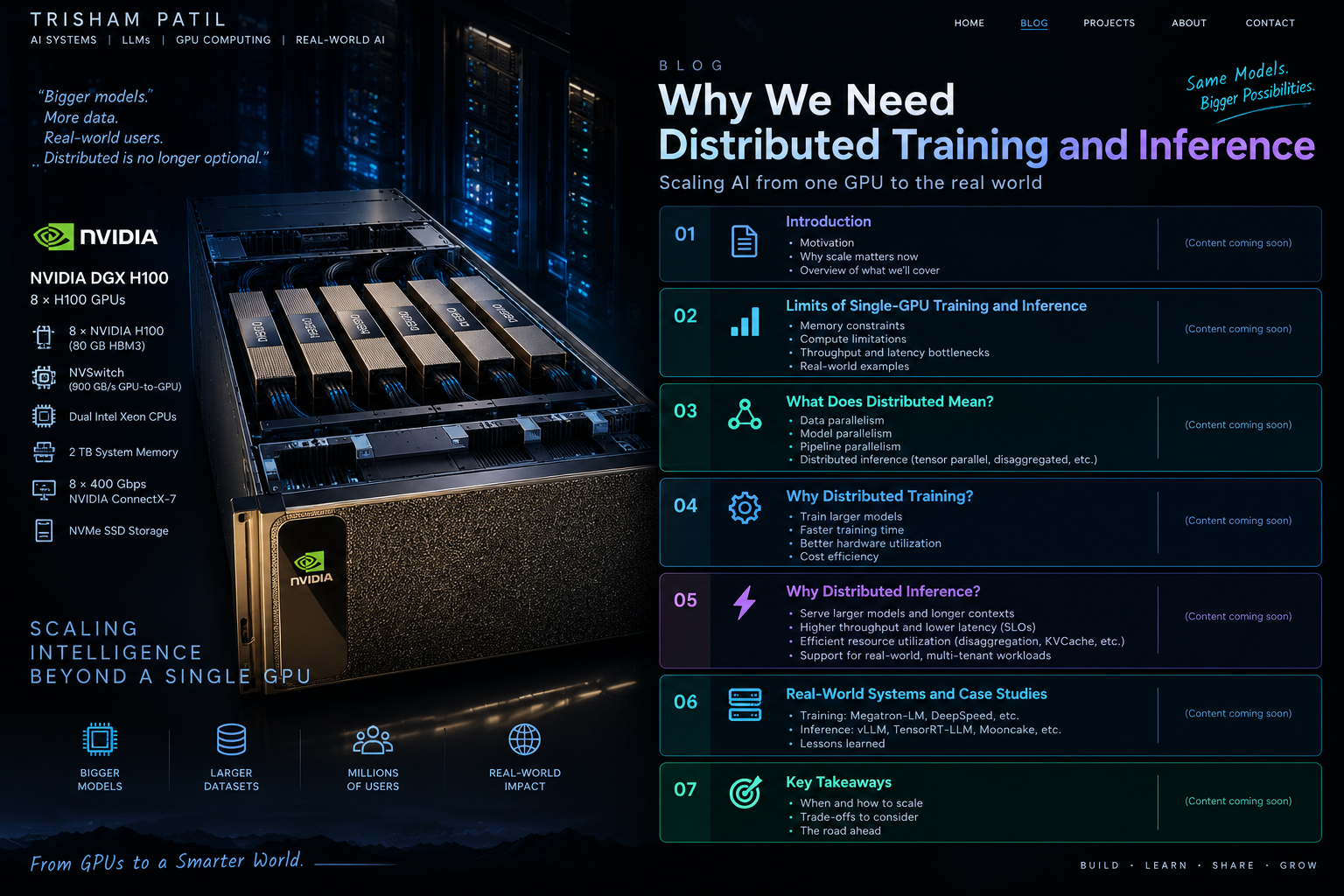
Introduction
Modern models have outgrown the hardware they run on. A single GPU can no longer hold a frontier model’s weights, chew through a multi-trillion-token dataset in reasonable time, or serve millions of low-latency requests. That is the whole reason distributed training and inference exists: not as a fancy optimization, but as the only way to make the math fit — across many GPUs, and across many machines.
This post is an engineering-first walk through why a single GPU stops being enough, what exactly gets split when you go distributed, and how those pieces are wired together in practice. We start from the four axes of parallelism, build up to 3D parallelism, then go deep on the workhorse of real clusters — PyTorch DistributedDataParallel (DDP) — with runnable code, the ring all-reduce that makes it scale, the NCCL interconnect ladder underneath it, the gotchas that silently corrupt runs, and a decision framework for picking DDP vs FSDP vs DeepSpeed vs Horovod.
The through-line: distributed training is a distributed-systems problem wearing a machine-learning costume. Once you see where the communication lives, most “why is my scaling worse than expected” questions answer themselves.
1. Why a Single GPU Is Not Enough
Why Distributed — The Math Doesn’t Fit Anymore
Distributed training is not a stylistic choice or a premature optimization. At modern AI scale, it becomes a hard requirement because the workload simply stops fitting into a single GPU — and it fails to fit along three independent axes: model size, dataset size, and wall-clock time. Any one of these is enough to force the issue; together they make single-GPU training impractical.
1. Model size — the weights may not even fit
The first wall is memory, and you hit it before you ever get to speed.
Consider a 70B parameter model in FP16. Storing just the weights requires roughly 140 GB (2 bytes per parameter × 70B). An H100-80GB offers 80 GB of GPU memory — so the model weights alone already exceed a single GPU’s capacity, with nothing left over.
And weights are only the beginning. Training is not just holding the model in memory; it also has to hold the optimizer states (for example, the moment estimates Adam maintains per parameter) and the activations produced during the forward pass and kept for the backward pass. These add substantially to the footprint, widening an already-impossible gap.
The key realization is subtle but important: the problem here is not that the model is computationally expensive. It is that the model and its training state do not physically fit inside a single GPU’s memory. No amount of patience makes 140+ GB fit into 80 GB.
2. Dataset size — the data takes too long
Even if the model did fit, the second wall is the sheer volume of data modern models are trained on.
A contemporary LLM pretraining budget can be on the order of 15 trillion tokens. Meanwhile, a single GPU training a 7B model might process only about 3–5 billion tokens per day. At that rate, pushing a ~15T-token budget through one GPU would take years — a training timeline that is completely unviable for any real project.
So distributed training is necessary not only because of how large the model is, but also because of how much data it must see. The dataset by itself makes single-GPU training impractical.
3. Wall-clock pressure — iteration has to be fast
The third wall is time-to-result, and it is about people and process as much as hardware.
Research progresses through iteration, and iteration needs to happen in days, not weeks. An experiment that might take around two weeks on a single GPU can be compressed into hours across a cluster by scaling the work over many GPUs. That difference is the gap between a fast feedback loop and a stalled one.
Distributed training, then, is also about reducing wall-clock time — making faster experimentation and iteration possible at all.
Putting it together
These three pressures compound into a single conclusion:
The model doesn’t fit → the dataset takes too long → the training timeline becomes unacceptable → therefore we need distributed training.
Single-GPU training does not fail because GPUs are slow. It fails because at modern AI scale the math no longer fits — not in memory, not in time. Everything that follows in this post is about how we spread the work across many GPUs to make it fit again.
2. The Scale of Modern AI Models
Four Axes to Parallelise Along
Once a model no longer fits comfortably on a single GPU, the natural next question is: what, exactly, do we split up? The important insight is that “distribute the work” is not a single operation. There are multiple independent dimensions of parallelism, and each one partitions a different part of the workload, requires a different kind of communication, and answers a different bottleneck.
The four fundamental axes are data, tensors, layers, and training state. Each keeps some things replicated and splits others across GPUs.
1. Data Parallelism
In data parallelism, every GPU holds a full replica of the model, and the batch is split across GPUs so each device processes a different slice of the data. Because each replica computes gradients on its own shard, the replicas must be kept in sync: this is done with an all-reduce of the gradients once per training step, after which every GPU applies the same update.
This is the default choice when the model already fits on each GPU and the goal is simply to increase throughput by processing more data in parallel.
2. Tensor Parallelism
Tensor parallelism attacks the opposite problem: a single layer that is too large for one GPU. Here the batch is replicated, but the weight tensors themselves are split — for example, partitioning a matrix by columns or by rows across devices. Because each GPU now computes only part of a layer’s output, the partial results must be combined with an all-reduce of activations inside each layer.
Use this when an individual layer does not fit on one GPU. The Megatron-LM style of sharding is the canonical example of this approach.
3. Pipeline Parallelism
Pipeline parallelism splits the model by layers, assigning different contiguous groups of layers to different GPUs, so the model is spread depth-wise across the cluster. Data then flows through this pipeline: GPUs communicate activations during the forward pass and gradients during the backward pass as work moves from one stage to the next.
This is the approach to reach for when the model is too deep to fit on a single GPU. GPipe and the 1F1B schedule are the associated examples.
4. Sharded (Fully Sharded Data Parallel (FSDP) / ZeRO Redundancy Optimizer)
The sharded approach targets memory directly. Instead of replicating the full model on every GPU, it splits the weights, gradients, and optimizer states across devices. The trade-off is communication: GPUs all-gather the weights when they are needed for computation and reduce-scatter the gradients afterward.
Use this when training is primarily memory-bound — when you cannot afford a full replica per GPU — while still wanting DDP-like training speed.
Comparing the four axes
The four approaches are best understood side by side — what each one splits, what it keeps replicated, the communication it introduces, and when it applies:
| Approach | What is split? | What is replicated? | Main communication | When to use |
|---|---|---|---|---|
| Data Parallelism | Batch | Model | Gradient all-reduce | Model fits; need throughput |
| Tensor Parallelism | Weight tensors | Batch | Activation all-reduce | Individual layer doesn’t fit |
| Pipeline Parallelism | Layers | — | Activations / gradients | Model is too deep |
| FSDP / ZeRO | Weights, gradients, optimizer states | — | All-gather / reduce-scatter | Memory-bound training |
The takeaway is that when one GPU is no longer enough, we are not limited to a single fix. We can distribute the workload along different axes — data, tensors, layers, or model/training state — and each axis is the right answer to a different reason the workload stopped fitting.
3D Parallelism — Combine All Three Axes
The four axes above are not mutually exclusive. Each one solves a different scaling problem — data parallelism buys throughput, tensor parallelism fits an oversized layer, pipeline parallelism fits an over-deep model — so at frontier scale you rarely pick just one. Instead, data parallelism, tensor parallelism, and pipeline parallelism are combined simultaneously into a single training topology. This composition is what is meant by 3D parallelism.
Combining the three dimensions
When all three are active at once, every GPU can be addressed by a (p, t, d) coordinate:
| Dimension | Symbol | What it represents |
|---|---|---|
| Pipeline | p | Pipeline stages |
| Tensor | t | Tensor-parallel partitions |
| Data | d | Data-parallel replicas |
The three sizes multiply to give the total number of GPUs. A concrete example:
\[4 \times 8 \times 4 = 128 \text{ GPUs}\]That configuration means the training run uses 4 pipeline stages, 8-way tensor parallelism, and 4-way data parallelism, for a total of 128 GPUs.
It helps to picture the topology as a cube:
- The data dimension spans across the columns.
- The tensor dimension spans across the rows.
- The pipeline dimension spans across the planes.
Every GPU sits at exactly one $(p, t, d)$ position in that cube, and its coordinate tells you which slice of the model, batch, and pipeline it is responsible for.
How to decide what parallelism to use
3D parallelism is powerful, but it is not the starting point — it is where you end up only when multiple constraints stack up. The decision sequence is:
- Start with DDP (plain data parallelism).
- If you hit a memory problem, move to FSDP or ZeRO-3.
- If one layer is too large to fit, add tensor parallelism.
- If the model is too deep to fit, add pipeline parallelism.
- When several of these constraints hold at once, combine the approaches into 3D parallelism.
A useful rule of thumb: pure FSDP alone can handle many cases for models under roughly 100B parameters. You reach for the full 3D combination when a single axis is no longer enough to make the workload fit and run efficiently.
Topology matters
Composing three dimensions is only half the story — where each dimension is placed on the hardware matters just as much, because the axes communicate at very different frequencies:
- Tensor-parallel ranks communicate at high frequency (an all-reduce inside every layer), so they should live on GPUs joined by high-bandwidth links such as NVLink.
- Pipeline stages exchange activations and gradients less often, so they can span nodes without paying a prohibitive cost.
- Data-parallel replicas synchronize only once per step, so they can span racks, where communication is comparatively low-frequency.
The key distinction is between communication frequency and hardware topology: you map the chattiest dimension onto the fastest interconnect, and let the less chatty dimensions stretch across the slower, longer links. Getting this mapping right is what makes a 3D-parallel system efficient rather than merely correct.
The broader point is that large-scale training does not force a choice of a single parallelism strategy. Multiple axes can be composed into one distributed topology, each addressing a different constraint, and arranged on the hardware according to how often they talk.
The Vocabulary of a Distributed Launcher
Before we can talk about how a distributed job starts up, we need the vocabulary a launcher uses to identify and coordinate every process. Whether you run 8 GPUs or 8,000, the launcher spins up a fleet of processes — typically one process per GPU — and each process needs to know two things: who am I in this job? and who do I talk to? A handful of terms answer both.
The hierarchy is worth holding in your head from the start:
Cluster → Nodes → GPUs → Processes → Ranks → Process Groups
A cluster contains nodes (machines); each node has several GPUs; each GPU is driven by a process; each process is assigned ranks that place it in the job; and process groups define which processes actually communicate together.
World Size
World size is the total number of distributed processes in the job. Since we typically launch one process per GPU, it is effectively the total GPU count.
For example, 2 nodes × 4 GPUs = world size 8. Throughout this section we’ll use that same 8-process job as the running example.
Global Rank
A rank is the unique identifier of a process across the entire distributed job. The global rank ranges from 0 to world_size - 1, and every process has a distinct one.
In our 8-process job, global ranks run 0..7, and a process might be, say, global rank 5 — its single address across the whole cluster.
Local Rank
The local rank is the process’s GPU index on its own node. It ranges from 0 to gpus_per_node - 1 and determines which GPU on the current node the process binds to.
With 4 GPUs per node, local ranks on each node run 0..3. A process with global rank 5 on the second node would have local rank 1 — meaning it binds to GPU 1 of that machine.
Node Rank and Process Group
Node rank identifies which machine the process is running on. It ranges from 0 to nnodes - 1. In our example there are 2 nodes, so node ranks are 0 and 1.
A process group defines the communicator — the set of processes that participate together in a collective communication operation. The default process group contains all ranks, i.e. every process in the job.
Together these draw a clean separation:
- Global rank — where this process sits in the entire job.
- Local rank — which GPU/process it corresponds to on its node.
- World size — how many processes participate in the job overall.
- Node rank — which machine the process belongs to.
- Process group — which processes communicate together.
Example Environment Variables
A launcher such as torchrun communicates all of this to each process through environment variables. For the process that is global rank 5 in our 8-process job:
RANK=5                    # global rank in [0, world_size)
LOCAL_RANK=1              # local rank in [0, gpus_per_node)
WORLD_SIZE=8              # total processes
MASTER_ADDR=node0.example.com
MASTER_PORT=29500
Reading these line by line:
RANK=5— this process’s global rank within the range[0, world_size).LOCAL_RANK=1— its local rank, i.e. the GPU index it binds to on its own node, within[0, gpus_per_node).WORLD_SIZE=8— the total number of processes in the job.MASTER_ADDR=node0.example.com— the address of the coordinating process the others use as a common reference point.MASTER_PORT=29500— the port on that address they connect to.
Every process in the job receives the same WORLD_SIZE, MASTER_ADDR, and MASTER_PORT, but its own RANK and LOCAL_RANK. That is precisely enough for each process to know its place in the job and where to reach the others — the foundation for how a distributed training job is actually launched and how these processes discover and communicate with one another.
Communication Backends
Knowing who each process is only gets you so far. Once the ranks are assigned, the processes still have to actually exchange data — moving gradients, activations, and parameters between GPUs and across nodes. That job is handled by a communication backend: the library that implements the collective communication underneath a distributed training job. Three backends come up in practice.
1. NCCL
NCCL — the NVIDIA Collective Communications Library — is the primary GPU-to-GPU communication backend for NVIDIA GPU training.
It is built to use the right hardware path automatically: within a node it can move data over NVLink, and across nodes it can use RDMA over InfiniBand (IB) or RoCE. Because it is topology-aware, it understands how the GPUs and links are physically arranged and routes traffic accordingly.
NCCL is the default choice for GPU training and is what almost all typical NVIDIA GPU distributed-training setups use.
2. Gloo
Gloo is a cross-platform communication backend originally developed at Facebook. It is CPU-friendly and portable, and it does not require special dependencies to run.
The trade-off is that it does not provide GPU acceleration the way NCCL does. That makes it most useful when debugging or running distributed workloads on CPU only, rather than as the production backend for GPU training.
3. MPI
MPI — the Message Passing Interface — is a standard widely used in HPC (high-performance computing) environments.
PyTorch supports MPI, but using it requires a rebuild/configuration with MPI support rather than working out of the box. Horovod can also use MPI underneath. MPI is particularly relevant when working with HPC clusters where MPI is already the established communication standard.
Choosing a backend in PyTorch
In PyTorch you select the backend when you initialize the process group:
dist.init_process_group(backend="nccl")
# 99.8% of the time, pick this.
For typical NVIDIA GPU distributed training, nccl is the backend to choose — the other two are for the specific situations described above (CPU/portable workloads for Gloo, HPC environments for MPI).
Comparison
| Backend | Primary use | GPU communication | Typical use |
|---|---|---|---|
| NCCL | NVIDIA GPU training | Yes | Production GPU training |
| Gloo | CPU / portable distributed workloads | No GPU acceleration | CPU debugging / CPU-only workloads |
| MPI | HPC / message passing | Depends on MPI implementation | HPC environments |
With the ranks assigned and a backend selected, we now have everything needed to look more closely at how distributed processes actually communicate.
Collective Primitives
A communication backend does not expose “send this gradient there” one message at a time. Instead it provides a small set of collective primitives — coordinated operations that involve all the ranks in a process group at once. Almost everything a distributed trainer does, from synchronizing initial weights to averaging gradients, is built out of these few operations. The easiest way to keep them straight is to track the direction of data flow: from one rank to many (1 → N), from many to one (N → 1), or from many to many (N → N).
1. Broadcast — (1 → N)
Broadcast sends data from one rank to all ranks. Everyone ends up with an identical copy of what the source rank held.
The canonical use is synchronizing initial weights from rank 0 to all ranks at the start of training, so every replica begins from exactly the same parameters.
2. Reduce — (N → 1)
Reduce combines data from all ranks — for example by summing — and delivers the result to one worker/rank.
The classic example is summing gradients to one worker. This is an older style of gradient aggregation, though, and is rarely used directly now in modern distributed training.
3. All-reduce — (N → N)
All-reduce combines data from all ranks and makes the resulting value available to all ranks — conceptually a reduce whose result is handed back to everyone.
In DDP, all-reduce is used for gradient synchronization: every replica contributes its local gradients and every replica walks away with the same averaged gradient. It is one of the fundamental communication primitives and a major workhorse of distributed training.
4. All-gather — (N → N)
All-gather collects data from all ranks so that every rank receives the complete gathered result — no reduction, just concatenation of everyone’s pieces onto everyone.
In FSDP, all-gather is used to regather sharded parameters before a forward or backward pass, temporarily reconstructing the full layer from the shards each rank holds.
5. Reduce-scatter — (N → N)
Reduce-scatter combines/reduces data across ranks and then distributes the resulting chunks so that each rank owns one reduced chunk — a reduction and a scatter fused into one step.
It can be viewed as the first half of a ring all-reduce, where each rank ends up owning one fully reduced chunk of the result.
6. Barrier
A barrier is not a data operation at all — it is a synchronization point. All workers wait until every rank has arrived at the barrier before any of them is allowed to proceed.
The key identity
There is one relationship worth committing to memory, because it ties several of these primitives together:
All-reduce = reduce-scatter followed by all-gather
That is: reduce-scatter first leaves each rank owning one fully reduced chunk, and all-gather then shares those chunks so every rank has the complete result. This decomposition is the conceptual foundation of ring all-reduce, which we will explore in more detail later.
Summary
| Primitive | Direction | Purpose / Example |
|---|---|---|
| Broadcast | 1 → N | Synchronize initial weights |
| Reduce | N → 1 | Aggregate gradients to one worker |
| All-reduce | N → N | DDP gradient synchronization |
| All-gather | N → N | FSDP parameter gathering |
| Reduce-scatter | N → N | Reduce and distribute chunks |
| Barrier | — | Synchronize all workers |
These six primitives are the basic vocabulary for how distributed training moves and synchronizes data across ranks — every parallelism strategy discussed earlier ultimately expresses its communication in terms of them.
Choosing the Right Parallelism Strategy
With the axes, the 3D combination, and the communication vocabulary all in hand, the practical question becomes: for a given workload, which strategies do I actually turn on? The answer scales with the job. The table below maps a few representative scenarios to the parallelism strategies they call for:
| Model / Scenario | Data Parallel | Tensor Parallel | Pipeline Parallel | Sharded |
|---|---|---|---|---|
| 7B fine-tune, 8 GPUs | Yes (DDP) | No | No | Optional (FSDP if tight) |
| 70B pretrain, 1 node (8×B200) | No | Yes (TP=8) | No | Yes (FSDP for opt state) |
| 70B pretrain, multi-node | Yes (across nodes) | Yes (within node) | Optional | Yes |
| GPT-4-class frontier model | Yes | Yes | Yes | Yes (all 4 combined) |
Read top to bottom, these rows describe a natural progression as the workload grows:
- A 7B fine-tuning workload on 8 GPUs can generally get by with plain data parallelism (DDP) — the model fits, so you just replicate it and split the batch. Sharding is optional, reached for only if memory turns out to be tight.
- A 70B pretraining workload on a single 8-GPU node no longer fits per GPU, so it turns to tensor parallelism across the GPUs (TP=8), with sharding used where necessary to hold the optimizer state.
- A 70B model across multiple nodes combines data parallelism across nodes with tensor parallelism within a node, and can introduce pipeline parallelism when appropriate — mapping each axis onto the level of the hardware that suits its communication frequency.
- At GPT-4-class frontier scale, all of the dimensions come together at once: data + tensor + pipeline + sharding, i.e. full 3D parallelism plus sharded state.
The central point is that there is no single parallelism strategy that is always correct. The right combination depends on model size, memory requirements, the number of GPUs, and whether the workload spans one node or many. The strategies introduced in this post are not competing options but a toolkit — you compose the subset that matches the constraints your workload actually hits.
From Parallelism Theory to a Working DDP Script
All the theory above answers what to split. The most common answer in practice — for anything from a single 8-GPU box to a 32-GPU job that still fits in memory — is the simplest one: data parallelism, implemented by PyTorch’s DistributedDataParallel (DDP). It is battle-tested, and it is what roughly 90% of teams reach for first.
The big idea behind DDP is deliberately unglamorous:
Write your single-GPU training loop. Wrap the model in DDP. Launch it with
torchrun. DDP handles the gradient synchronization for you.
To see how little changes, start from the single-GPU baseline the DDP version has to match.
The single-GPU baseline
train_single.py is an ordinary ResNet-18 on CIFAR-10 — no distributed machinery at all. It is the pedagogical control: the DDP version must produce equivalent training, just faster.
# train_single.py — single-GPU baseline (the control case)
import torch
import torch.nn as nn
from torch.utils.data import DataLoader
from torchvision import datasets, transforms, models


def main():
    device = torch.device("cuda:0" if torch.cuda.is_available() else "cpu")

    transform = transforms.Compose([
        transforms.ToTensor(),
        transforms.Normalize((0.4914, 0.4822, 0.4465),
                             (0.2470, 0.2435, 0.2616)),
    ])
    train_set = datasets.CIFAR10(root="./data", train=True,
                                 download=True, transform=transform)
    train_loader = DataLoader(train_set, batch_size=128,
                              shuffle=True, num_workers=4, pin_memory=True)

    model = models.resnet18(num_classes=10).to(device)
    optimizer = torch.optim.SGD(model.parameters(), lr=0.1, momentum=0.9)
    criterion = nn.CrossEntropyLoss()

    for epoch in range(3):
        model.train()
        for images, labels in train_loader:
            images, labels = images.to(device), labels.to(device)
            optimizer.zero_grad()
            loss = criterion(model(images), labels)
            loss.backward()
            optimizer.step()
        print(f"epoch {epoch} done")

    torch.save(model.state_dict(), "resnet18_cifar10.pt")


if __name__ == "__main__":
    main()
Note the three things that will have to change for DDP: the DataLoader uses shuffle=True (a single process owns the whole dataset), there is no notion of a “rank,” and the save is a plain state_dict().
The DDP version
train_ddp.py is the same training loop with the distributed scaffolding added. Read it against the baseline — the loop body is unchanged; everything new is setup, sharding, and rank-aware bookkeeping.
# train_ddp.py — single-node multi-GPU DDP (launch with torchrun)
import os
import argparse
import torch
import torch.nn as nn
import torch.distributed as dist
from torch.nn.parallel import DistributedDataParallel as DDP
from torch.utils.data import DataLoader
from torch.utils.data.distributed import DistributedSampler
from torchvision import datasets, transforms, models


def ddp_setup():
    """torchrun sets RANK / LOCAL_RANK / WORLD_SIZE for us."""
    dist.init_process_group(backend="nccl")          # blocking rendezvous
    local_rank = int(os.environ["LOCAL_RANK"])
    torch.cuda.set_device(local_rank)                # bind BEFORE touching the GPU
    return int(os.environ["RANK"]), local_rank, int(os.environ["WORLD_SIZE"])


def ddp_cleanup():
    dist.destroy_process_group()


def is_rank_zero():
    return int(os.environ.get("RANK", 0)) == 0


def log0(*args):
    if is_rank_zero():
        print(*args, flush=True)


def build_model(local_rank):
    model = models.resnet18(num_classes=10)
    # Small per-GPU batches make per-device BatchNorm stats noisy — sync them.
    model = nn.SyncBatchNorm.convert_sync_batchnorm(model)
    return model.to(local_rank)


def build_loaders(per_gpu_batch_size, rank, world_size):
    transform = transforms.Compose([
        transforms.ToTensor(),
        transforms.Normalize((0.4914, 0.4822, 0.4465),
                             (0.2470, 0.2435, 0.2616)),
    ])
    # Only rank 0 downloads; everyone else waits at the barrier.
    if is_rank_zero():
        datasets.CIFAR10(root="./data", train=True, download=True)
    dist.barrier()

    train_set = datasets.CIFAR10(root="./data", train=True,
                                 download=False, transform=transform)
    sampler = DistributedSampler(train_set, num_replicas=world_size,
                                 rank=rank, shuffle=True, drop_last=True)
    loader = DataLoader(train_set, batch_size=per_gpu_batch_size,
                        sampler=sampler, num_workers=4,
                        pin_memory=True, drop_last=True)
    return loader, sampler


@torch.no_grad()
def evaluate(model, loader, local_rank):
    model.eval()
    loss_sum = torch.zeros(1, device=local_rank)
    correct = torch.zeros(1, device=local_rank)
    total = torch.zeros(1, device=local_rank)
    criterion = nn.CrossEntropyLoss(reduction="sum")
    for images, labels in loader:
        images, labels = images.to(local_rank), labels.to(local_rank)
        logits = model(images)
        loss_sum += criterion(logits, labels)
        correct += (logits.argmax(1) == labels).sum()
        total += labels.numel()
    # Reduce metrics across all ranks so every process agrees.
    for t in (loss_sum, correct, total):
        dist.all_reduce(t, op=dist.ReduceOp.SUM)
    return (loss_sum / total).item(), (correct / total).item()


def main():
    parser = argparse.ArgumentParser()
    parser.add_argument("--epochs", type=int, default=3)
    parser.add_argument("--per-gpu-batch-size", type=int, default=128)
    parser.add_argument("--base-lr", type=float, default=0.1)
    args = parser.parse_args()

    rank, local_rank, world_size = ddp_setup()

    # Linear LR scaling rule (Goyal et al., 2017): scale LR with global batch.
    reference_batch = 128
    global_batch = args.per_gpu_batch_size * world_size
    scaled_lr = args.base_lr * global_batch / reference_batch

    model = DDP(build_model(local_rank), device_ids=[local_rank])
    loader, sampler = build_loaders(args.per_gpu_batch_size, rank, world_size)
    optimizer = torch.optim.SGD(model.parameters(), lr=scaled_lr, momentum=0.9)
    criterion = nn.CrossEntropyLoss()

    for epoch in range(args.epochs):
        model.train()
        sampler.set_epoch(epoch)          # CRITICAL: reshuffles each epoch
        for images, labels in loader:
            images, labels = images.to(local_rank), labels.to(local_rank)
            optimizer.zero_grad()
            loss = criterion(model(images), labels)
            loss.backward()               # all-reduce of gradients fires here
            optimizer.step()
        log0(f"epoch {epoch} done | lr={scaled_lr:.4f}")

    if is_rank_zero():
        # Unwrap .module so the checkpoint has no "module." prefix.
        torch.save(model.module.state_dict(), "resnet18_cifar10_ddp.pt")

    ddp_cleanup()


if __name__ == "__main__":
    main()
Four lines carry the entire distributed story:
dist.init_process_group(backend="nccl")— the blocking rendezvous where all ranks find each other.DistributedSampler(...)+sampler.set_epoch(epoch)— gives each rank a disjoint shard and reshuffles it every epoch.DDP(model, device_ids=[local_rank])— registers a backward hook that all-reduces gradients automatically duringloss.backward().model.module.state_dict()— saved only from rank 0, unwrapping the DDP wrapper.
Launching it on one node
You do not run python train_ddp.py. You hand it to torchrun, which spawns one process per GPU and injects RANK / LOCAL_RANK / WORLD_SIZE:
# Two GPUs, one machine.
torchrun --standalone --nproc_per_node=2 train_ddp.py \
    --epochs 3 --per-gpu-batch-size 128
That single command is the whole “launch step” of the big idea.
Launching DDP Across Nodes
Multi-node is the same script — only the launch changes. Every node runs its own torchrun, they all agree on a rendezvous endpoint, and NCCL wires the ranks together.
#!/usr/bin/env bash
# launch_multinode.sh — run on EACH node (differing NODE_RANK)
set -euo pipefail

: "${MASTER_ADDR:?set MASTER_ADDR to node 0's address}"
: "${NODE_RANK:?set NODE_RANK (0 for the first node)}"

NNODES="${NNODES:-2}"
MASTER_PORT="${MASTER_PORT:-29500}"
NPROC_PER_NODE="${NPROC_PER_NODE:-$(nvidia-smi --list-gpus | wc -l)}"
JOB_ID="${JOB_ID:-ddp-job-001}"

# --- NCCL tuning (uncomment as needed; see the env-var table below) ---
# export NCCL_DEBUG=INFO
# export NCCL_SOCKET_IFNAME=eth0
# export NCCL_IB_HCA=mlx5_0,mlx5_1
# export NCCL_P2P_DISABLE=0
# export NCCL_ASYNC_ERROR_HANDLING=1

torchrun \
    --nnodes="${NNODES}" \
    --nproc_per_node="${NPROC_PER_NODE}" \
    --node_rank="${NODE_RANK}" \
    --rdzv_id="${JOB_ID}" \
    --rdzv_backend=c10d \
    --rdzv_endpoint="${MASTER_ADDR}:${MASTER_PORT}" \
    --max_restarts=3 \
    ../02_ddp_single_node/train_ddp.py --epochs 3 --per-gpu-batch-size 128
How N processes on K machines find each other
The --rdzv_backend=c10d flag selects PyTorch’s collective-communications rendezvous. The handshake is worth knowing, because most multi-node failures happen right here:
- Each process starts knowing its own rank, the total
world_size, and a masteraddr:port. - Rank 0 opens a TCP store on
MASTER_ADDR:MASTER_PORTand waits for connections. - All other ranks connect to the store and register themselves.
- Once
world_sizeprocesses have registered, they exchange a NCCL unique ID through the store. - NCCL uses that ID to set up peer-to-peer communicators between all ranks.
- The first collective runs, NCCL picks a ring topology, and training starts.
When it hangs: a rendezvous timeout almost always means a firewall is blocking
MASTER_PORT, the wrongMASTER_ADDR, or ranks disagreeing onworld_size. Runtelnet node0 29500from each node before blaming the model.
NCCL environment variables you’ll actually use
| Variable | Example value | What it does |
|---|---|---|
NCCL_DEBUG |
INFO |
Verbose logs. Set during bring-up; turn off in production (spammy). |
NCCL_SOCKET_IFNAME |
eth0 / ^lo,docker0 |
Which network interface to use — essential with multiple NICs. |
NCCL_IB_HCA |
mlx5_0,mlx5_1 |
Pin to specific InfiniBand HCAs. Prevents slow fallback. |
NCCL_IB_DISABLE |
1 |
Force TCP fallback — use to confirm IB is the culprit. |
NCCL_ASYNC_ERROR_HANDLING |
1 |
Errors become exceptions instead of deadlocks. Highly recommended. |
NCCL_BUFFSIZE |
8388608 |
Bytes per collective chunk. Tune for small-message-heavy workloads. |
The DDP Memory Footprint
DDP replicates the full model on every GPU, so before you launch, do the memory arithmetic. For a 7B-parameter model trained with AdamW and an FP32 master copy, one rank looks roughly like this:
| Component | Footprint (7B) | Where it comes from |
|---|---|---|
| Weights | ~14 GB | 2 bytes/param (FP16) × 7B |
| Gradients | ~14 GB | one gradient per weight |
| Optimizer states | ~56 GB | AdamW momentum + variance + FP32 master |
| Activations | ~10–40 GB | depends on batch size and sequence length |
| Total per rank | ~84–124 GB | × N ranks (DDP replicates everything) |
The punchline: DDP does not save memory — it multiplies it. Every rank pays the full ~84–124 GB. The moment that total exceeds your GPU (an 80 GB H100, say), plain DDP is off the table and you move to FSDP/ZeRO, which shard exactly the weights, gradients, and optimizer states this table enumerates.
Ring All-Reduce: Why Communication Doesn’t Explode as GPUs Grow
DDP’s one piece of communication is the gradient all-reduce after every backward pass. The obvious worry: as you add GPUs, does that all-reduce get more expensive per GPU? If it did, distributed training would die at a handful of GPUs. It doesn’t — and the reason is the algorithm NCCL uses.
Naive vs. ring
- Naive all-reduce: every GPU sends its gradient to every other GPU. With
NGPUs and a gradient ofMbytes, per-GPU traffic isO(N·M). Doubling GPUs doubles per-GPU communication — this collapses around ~8 GPUs. - Ring all-reduce (what NCCL does): GPUs form a logical ring, each talking only to its two neighbours. Per-GPU traffic is
2·(N-1)/N · M, which approaches2MasN → ∞— independent of cluster size.
That independence is the whole game: 8 GPUs cost the same communication per GPU as 1024 GPUs. It is the algorithmic foundation of scaling to thousands of GPUs.
The algorithm
Split each gradient into N chunks and run two phases, each N-1 steps:
- Reduce-scatter. At step
k, each GPU sends chunk(rank - k) mod Nto its right neighbour, which sums it with its own. AfterN-1steps, each GPU holds exactly one fully-summed chunk. - All-gather. Each GPU passes its fully-summed chunk around the ring. After
N-1more steps, every GPU has the complete sum.
This is the same identity introduced earlier — all-reduce = reduce-scatter + all-gather — realized on a ring. The per-GPU bandwidth cost is:
\[\text{cost} = 2 \cdot \frac{N-1}{N} \cdot M\]| GPUs (N) | Per-GPU cost |
|---|---|
| 2 | 1.00 · M |
| 4 | 1.50 · M |
| 8 | 1.75 · M |
| 1024 | ~2.00 · M |
Measuring it yourself
allreduce_benchmark.py sweeps message sizes and reports achieved bandwidth per rank, using exactly the 2·(N-1)/N factor to convert wall time into effective bandwidth:
# allreduce_benchmark.py — NCCL all-reduce bandwidth sweep
# Launch: torchrun --standalone --nproc_per_node=<GPUs> allreduce_benchmark.py
import os
import torch
import torch.distributed as dist


def bench(size_bytes, iters=50, warmup=5):
    world = dist.get_world_size()
    n_elems = size_bytes // 4                     # fp32 = 4 bytes
    x = torch.ones(n_elems, dtype=torch.float32, device="cuda")

    for _ in range(warmup):
        dist.all_reduce(x)
    torch.cuda.synchronize()

    start = torch.cuda.Event(enable_timing=True)
    end = torch.cuda.Event(enable_timing=True)
    start.record()
    for _ in range(iters):
        dist.all_reduce(x)
    end.record()
    torch.cuda.synchronize()

    sec = start.elapsed_time(end) / 1000.0 / iters
    # Ring all-reduce moves 2*(N-1)/N * M bytes per rank.
    factor = 2 * (world - 1) / world
    gb_per_s = (factor * size_bytes) / sec / 1e9
    return gb_per_s


def main():
    dist.init_process_group(backend="nccl")
    torch.cuda.set_device(int(os.environ["LOCAL_RANK"]))
    rank = dist.get_rank()

    if rank == 0:
        print(f"{'size':>12} {'bandwidth (GB/s/rank)':>24}")
    for log2_size in range(12, 30):               # 4 KiB .. 512 MiB
        size = 1 << log2_size
        bw = bench(size)
        if rank == 0:
            print(f"{size:>12} {bw:>24.2f}")

    dist.destroy_process_group()


if __name__ == "__main__":
    main()
Small messages will look slow (latency-bound); large messages converge on the interconnect’s real bandwidth. Which brings us to what that interconnect actually is.
NCCL Is Topology-Aware
NCCL does not use one fixed path. At init it probes CUDA_VISIBLE_DEVICES, reads the NVML topology, and discovers NICs — building a graph of which GPUs share NVLink, which share a PCIe root, and which NICs sit close to which GPUs — then picks the fastest ring that visits every rank. You can see its choice in NCCL_DEBUG=INFO output.
| Scope | Transport | Character |
|---|---|---|
| Intra-node | NVLink | Direct GPU-to-GPU, ~900 GB/s on H100 |
| NVSwitch | Full-bandwidth all-to-all in HGX boxes | |
| PCIe P2P | Direct GPU-GPU over PCIe, ~50 GB/s | |
| Inter-node | InfiniBand + GPUDirect | Zero-copy GPU↔NIC. Best. |
| RoCEv2 + GPUDirect | RDMA over Ethernet, near-IB | |
| Sockets (TCP) | Fallback. 5–10× slower. |
The bandwidth ladder
Every hop away from the GPU die costs roughly an order of magnitude. Knowing where your job sits on this ladder explains most “why is scaling worse than expected” surprises:
| Interconnect | Approx. bandwidth |
|---|---|
| NVLink 5 (B200, intra-node) | ~1.8 TB/s |
| NVSwitch (HGX, all-to-all) | ~900 GB/s |
| InfiniBand NDR (inter-node) | ~400–800 Gb/s |
| RoCEv2 Ethernet (inter-node) | ~200–400 Gb/s |
| PCIe Gen5 P2P (fallback) | ~64 GB/s |
| TCP sockets (last resort) | ~10–25 Gb/s |
This is also why 3D-parallel topology mapping matters: you pin the chattiest dimension (tensor parallelism) to NVLink and let the quiet dimension (data parallelism) stretch across the slower inter-node links.
The Five DDP Gotchas
DDP is simple to run and easy to run wrong. These five bugs are silent — the job doesn’t crash, it just trains worse — which is exactly what makes them worth memorizing.
- Forgot
sampler.set_epoch(epoch). Every epoch reuses the same shuffle, so each rank sees the identical order forever. Accuracy quietly suffers. Fix: callset_epoch(epoch)at the top of every epoch. - Saved
model.state_dict()instead ofmodel.module.state_dict(). The checkpoint gets amodule.prefix on every key and won’t load into a plain model. Fix: unwrap.moduleand save from rank 0 only. - BatchNorm on tiny per-GPU batches. With per-GPU batch < ~16, per-device BN statistics are noisy — measurably worse accuracy (~4% in the notes’ example). Fix:
nn.SyncBatchNorm.convert_sync_batchnorm(model). - Uneven final batch → hang. If one rank gets a smaller last batch, collectives desynchronize and the job deadlocks. Fix:
drop_last=Trueon both the sampler and the loader. find_unused_parameters=Trueas a crutch. It papers over model-graph bugs at a 10–20% throughput cost. Fix: find the genuinely unused parameters and fix the forward pass instead of leaving the flag on.
Scaling: Strong vs. Weak, and Where Efficiency Goes
Two scaling questions
- Strong scaling — fixed problem, more GPUs. Does my existing job finish faster on 8 GPUs than on 2? Ideal time is
1/N; reality runs into communication floors. Matters for eval sweeps, research iteration, deadlines. - Weak scaling — fixed per-GPU work, more GPUs. If I scale to a bigger problem, does wall time stay constant? Ideal is constant time; communication adds overhead.
Most real AI workloads are weak scaling — we spend extra compute on training bigger things, not on finishing the same job faster.
Where the missing efficiency goes
When a job scales worse than N×, the loss is not mysterious. A representative breakdown of GPU time:
| Category | Time | How to attack it |
|---|---|---|
| Useful compute | 64% | — |
| All-reduce (not overlapped) | 12% | Larger model / smaller buckets / bigger grad accumulation |
| Stragglers (slow GPUs) | 10% | Homogeneous nodes; pin to healthy GPUs |
| Load imbalance | 6% | Even sharding; same-shape inputs (pad or drop) |
| Host overhead | 4% | Fewer Python callbacks; compiled model |
| Data-loading stalls | 4% | pin_memory=True, prefetch, more num_workers |
Measure first. The PyTorch profiler plus
torch.cuda.Eventgive you the actual breakdown. Don’t guess which bar is tallest — profile and attack the biggest one.
Optimization levers, in order of ROI
- Mixed precision (AMP) — fp16/bf16 halves memory and bandwidth for a 1.5–2× speedup. Should be on by default.
- Larger per-GPU batch + gradient accumulation — amortizes the all-reduce across more work. The dominant lever for communication efficiency.
- Tune NCCL bucket size/count — default 25 MB. Large models like bigger buckets; small models like more, smaller ones.
- Gradient compression (PowerSGD, signSGD) — rare but powerful: 10–100× less traffic for a small accuracy hit.
- Hierarchical (tree) all-reduce — NCCL picks this automatically on clustered topologies. Nothing to tune.
- Overlap opt-step with the next batch’s comm — advanced; most of the gain is already captured by DDP’s backward hook.
Putting a number on it
Scaling efficiency is a single ratio:
\[\text{eff}(N) = \frac{\text{throughput}(N)}{N \cdot \text{throughput}(1)}\]With a 420 samples/sec single-GPU baseline and 3,190 samples/sec on 8 GPUs:
\[\text{eff}(8) = \frac{3190}{8 \times 420} = \frac{3190}{3360} \approx 0.949\]94.9% at 8 GPUs is excellent — well-tuned DDP jobs on NVLink+IB clusters typically land in the 85–95% range. Below ~80%, profile immediately; above ~95%, you’re likely compute-bound and further tuning has diminishing returns. Always report both throughput and efficiency — throughput alone hides whether you’re wasting GPU-hours.
benchmark_scaling.py measures this end-to-end on synthetic data, so you can characterize a cluster before committing a real run to it:
# benchmark_scaling.py — DDP scaling-efficiency micro-benchmark (ResNet-50)
# Launch on N GPUs, compare global samples/s against the N=1 baseline.
import os
import time
import torch
import torch.nn as nn
import torch.distributed as dist
from torch.nn.parallel import DistributedDataParallel as DDP
from torchvision import models

WARMUP_STEPS = 10
MEASURE_STEPS = 100
PER_GPU_BATCH = 64
INPUT_SHAPE = (3, 224, 224)


def main():
    dist.init_process_group(backend="nccl")
    local_rank = int(os.environ["LOCAL_RANK"])
    torch.cuda.set_device(local_rank)
    world = dist.get_world_size()

    model = DDP(models.resnet50().to(local_rank), device_ids=[local_rank])
    optimizer = torch.optim.SGD(model.parameters(), lr=0.1)
    criterion = nn.CrossEntropyLoss()

    x = torch.randn(PER_GPU_BATCH, *INPUT_SHAPE, device=local_rank)
    y = torch.randint(0, 1000, (PER_GPU_BATCH,), device=local_rank)

    def step():
        optimizer.zero_grad()
        loss = criterion(model(x), y)
        loss.backward()
        optimizer.step()

    for _ in range(WARMUP_STEPS):
        step()
    torch.cuda.synchronize()

    start = time.perf_counter()
    for _ in range(MEASURE_STEPS):
        step()
    torch.cuda.synchronize()
    elapsed = time.perf_counter() - start

    local_sps = (MEASURE_STEPS * PER_GPU_BATCH) / elapsed
    t = torch.tensor([local_sps], device=local_rank)
    dist.all_reduce(t, op=dist.ReduceOp.SUM)         # global throughput
    global_sps = t.item()

    if dist.get_rank() == 0:
        print(f"world_size={world}  global={global_sps:,.0f} samples/s "
              f"({global_sps / world:,.0f}/GPU)")
        print("Compare to N=1: eff(N) = global(N) / (N * global(1)). "
              "Below ~0.85 => interconnect-limited, comm-dominated, "
              "or stragglers.")

    dist.destroy_process_group()


if __name__ == "__main__":
    main()
Picking the Right Tool: DDP vs. FSDP vs. DeepSpeed vs. Horovod
DDP is the default, not the only option. The moment the memory table above overflows your GPU, you graduate to a sharding framework. Here is the honest comparison:
| Framework | Memory efficiency | Setup | Speed (fits-in-memory) | Framework support |
|---|---|---|---|---|
| DDP | Low (full replica) | Low | Fastest | PyTorch only |
| FSDP | High (full shard) | Medium | Near-DDP with overlap | PyTorch-native |
| DeepSpeed ZeRO | Highest (+ CPU offload) | Medium–High | Comparable to FSDP | PyTorch (via plugin) |
| Horovod | Low (full replica) | Medium | Comparable to DDP | PyTorch, TF, MXNet |
A decision framework
| Scenario | Pick | Why |
|---|---|---|
| 7B model, 8–32 GPUs, fits in memory | DDP | Simplest, battle-tested — what most teams use |
| 13–70B, memory-tight but per-layer fits | FSDP | Shards weights + grads + opt state; keeps DDP’s simplicity |
| Very tight memory, want library-level knobs | DeepSpeed ZeRO-3 | More knobs than FSDP; CPU-offload options |
| Existing TF/MXNet codebase on an HPC cluster | Horovod | Framework-portable; plays nicely with MPI + Slurm |
| A single layer doesn’t fit on one GPU | Tensor Parallel (Megatron) | Can’t split the batch — must split the weights |
| Trillion-parameter frontier model | 3D Parallel (Megatron-DeepSpeed) | Combine data + tensor + pipeline |
The one-line heuristic: When in doubt, DDP. When it OOMs, FSDP. When those aren’t enough, you’re at frontier scale — and back in the 3D-parallelism territory from the first half of this post.
Horovod, briefly
Horovod is Uber’s 2017 library. It uses MPI (not c10d) for rendezvous and NCCL for collectives, and it is framework-agnostic (TF, PyTorch, MXNet), launched with horovodrun. Its activity has declined since PyTorch shipped first-class DDP, but it still wins for an existing TensorFlow codebase, an HPC cluster where Slurm + MPI is already set up, or a training script that must stay framework-portable. The shape of a Horovod script:
import horovod.torch as hvd

hvd.init()                                    # instead of dist.init_process_group
torch.cuda.set_device(hvd.local_rank())

optimizer = torch.optim.Adam(model.parameters(), lr=1e-3)
optimizer = hvd.DistributedOptimizer(         # instead of the DDP wrap
    optimizer, named_parameters=model.named_parameters())

hvd.broadcast_parameters(model.state_dict(), root_rank=0)
hvd.broadcast_optimizer_state(optimizer, root_rank=0)
# Training loop — identical to DDP.
# Launch: horovodrun -np 8 -H node0:4,node1:4 python train.py
Key Takeaways
- A single GPU stops being enough along three axes — model size, dataset size, and wall-clock time — and any one of them is sufficient to force distribution.
- There are four ways to split the work — data, tensor, pipeline, and sharded (FSDP/ZeRO) — and at frontier scale you compose them into 3D parallelism, mapped onto hardware by communication frequency.
- DDP is the workhorse: write the single-GPU loop, wrap in DDP, launch with
torchrun. The gradient all-reduce is the only communication, and it fires insideloss.backward(). - Ring all-reduce is why this scales — per-GPU cost is
2·(N-1)/N·M, independent of cluster size, so 8 GPUs cost the same per-GPU comm as 1024. - DDP replicates memory, it doesn’t save it — a 7B AdamW run is ~84–124 GB per rank. When that overflows, move to FSDP or ZeRO.
- Most scaling losses are diagnosable — profile first, then attack unoverlapped all-reduce, stragglers, and load imbalance in that order. Report both throughput and efficiency.
Conclusion
Distributed training is less a machine-learning trick than a distributed-systems discipline: assign ranks, choose a backend, express your work as collective primitives, and map the chattiest communication onto the fastest interconnect. Everything from the four parallelism axes down to a single torchrun command is in service of one goal — making a workload that no longer fits on one GPU fit across many, without letting communication eat the gains.
Start simple. Reach for DDP, measure your scaling efficiency, and only add sharding, tensor, or pipeline parallelism when a concrete constraint forces you to. The frontier-scale machinery is impressive, but the engineering judgment that matters most is knowing the smallest tool that solves the problem in front of you.
If training is about surviving scale, the natural sequel is distributed inference — serving those trained models under latency and throughput pressure, where the KV cache, request batching, and model sharding raise a fresh set of distributed-systems questions. That is a story for its own post.