Maximal Update Parameterization (μP): Hyperparameter Transfer Across Model Width — and Why It Isn't Free
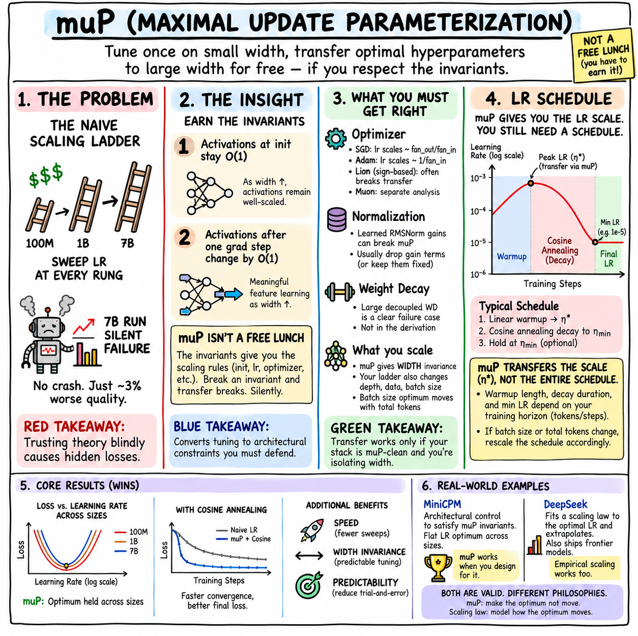
There is a line you hear constantly around large-model training: “just use μP — tune the learning rate once on a small model and transfer it to the big one for free.”
That statement is directionally right and operationally dangerous. Maximal Update Parameterization (μP) is real, it works, and it can save an enormous amount of compute. But it is not a learning-rate transfer trick, and treating it like one is exactly how teams end up with a 7B model that is quietly 3% worse than it should be, with a training curve that looks perfectly healthy and no obvious reason why.
This post unpacks what μP actually does, from first principles: the problem it solves, the two invariants it enforces, why the correct scaling depends on your optimizer, the implementation details that silently break it, and where it stops — because μP solves the width dimension of scaling and nothing else. By the end you should be able to reason about μP as an engineering constraint you have to earn, not a formula you get for free.
The Problem: Sweeping Hyperparameters at Every Size Is Expensive
Say you are building a family of models:
100M → 500M → 1B → 7B → 30B
Under ordinary parameterization, the optimal learning rate moves as the model gets wider. You might sweep and find:
100M     LR = 3e-4
500M     LR = 2e-4
1B       LR = 1e-4
7B       LR = 4e-5
Every rung on that ladder is its own hyperparameter sweep, and the sweeps get ruinously expensive as the models grow. You cannot afford to grid-search learning rates at 30B.
The question μP asks is:
Can we parameterize increasingly wide networks so that their training behavior stays comparable as width increases?
If the answer is yes, then in principle:
100M model
   ↓ sweep LR once
find LR = 3e-4
   ↓
1B  ──────────→ use the μP-consistent LR
7B  ──────────→ use the μP-consistent LR
That is the hyperparameter transfer idea (μTransfer). But notice the load-bearing word is transferability under a parameterization — not “the learning rate is invariant.” Keep that distinction; the whole post hangs on it.
Why Ordinary Parameterization Breaks as You Scale Width
Start with a single linear layer of width $n$:
\[y = Wx, \qquad y_i = \sum_{j=1}^{n} W_{ij}\,x_j\]Each output $y_i$ is a sum of $n$ terms. If every term has roughly constant variance, then
\[\mathrm{Var}(y_i) \sim n\]which explodes as the network gets wider. That is why standard initialization scales the weights down:
\[W_{ij} \sim \mathcal{O}\!\left(\frac{1}{\sqrt{n}}\right)\]so the sum stays $\mathcal{O}(1)$ regardless of width. This is the familiar Kaiming/Xavier logic, and it keeps activations well-behaved at initialization.
But here is the catch: initialization stability is only half the story.
Initialization Isn’t Enough — You Also Need Meaningful Updates
Keeping activations sane at step 0 is necessary but not sufficient. You also want training to actually change those activations by a meaningful amount as width grows.
Concretely, suppose an activation starts at:
activation = 1.0
After a gradient step, you want something like:
activation = 1.0 + O(1) ✅ meaningful update
not:
activation = 1.0 + 0.000001  ❌ lazy — features barely move
activation = 1.0 + 1000      ❌ unstable — training blows up
So μP enforces two invariants simultaneously:
\[h = \mathcal{O}(1) \quad\text{(activations stay bounded)}\] \[\Delta h = \mathcal{O}(1) \quad\text{(activations change meaningfully per step)}\]That second invariant is the heart of it. It says the network must keep learning features at the same effective rate no matter how wide it gets.
Why “Feature Learning” Is the Whole Point
Imagine widening a network and, to stay numerically safe, shrinking the updates as you go:
100 neurons     → update = 0.1
1,000 neurons   → update = 0.01
10,000 neurons  → update = 0.001
Everything is stable. But the wider model has become lazy — its features barely move during training. In the infinite-width limit this is the “kernel” or “lazy training” regime, where the network stops learning representations and behaves like a fixed feature map.
μP wants the opposite:
100 neurons       → meaningful feature change
1,000 neurons     → meaningful feature change
10,000 neurons    → meaningful feature change
1,000,000 neurons → meaningful feature change
That is what “maximal update” means: the largest per-step feature update you can take while remaining stable. Enforce that, and wide models keep learning like their small counterparts — which is precisely why their optimal hyperparameters line up.
From Two Invariants to Concrete Scaling Rules
Here is the clever part. Once you commit to:
activations $\mathcal{O}(1)$, and their per-step change $\mathcal{O}(1)$
you can derive how everything else must scale with width. μP gives you coordinated rules for:
- initialization variance,
- learning rates (per parameter group),
- the magnitude of parameter updates,
- output/readout layers,
- embeddings,
- hidden weights.
flowchart TD
    I1["Invariant 1<br/>activations = O(1)"] --> D[Derive width-scaling rules]
    I2["Invariant 2<br/>Δactivations = O(1)"] --> D
    D --> P[parameter init scaling]
    D --> L[learning-rate scaling]
    D --> U[update-magnitude scaling]
    P --> DYN[Preserved training dynamics]
    L --> DYN
    U --> DYN
    DYN --> T[Width-transferable hyperparameters]

    style I1 fill:#dbeafe,stroke:#3b82f6
    style I2 fill:#dbeafe,stroke:#3b82f6
    style DYN fill:#fef9c3,stroke:#eab308
    style T fill:#dcfce7,stroke:#22c55e
And critically:
The correct learning-rate scaling depends on the optimizer.
μP does not hand you a single universal “keep LR constant” rule. It tells you how the effective update should scale with width, and the parameterization needed to achieve that differs by optimizer.
Optimizer Matters: SGD vs Adam vs Lion
SGD. The update is proportional to the raw gradient:
\[\Delta W = -\eta\, \nabla_W L\]The gradient’s scaling with width depends on where the parameter sits in the network, so μP derives an LR scaling for each parameter group accordingly.
Adam. The update is normalized by the second-moment estimate:
\[\Delta W = -\eta\, \frac{m_t}{\sqrt{v_t} + \epsilon}\]Because Adam divides out the gradient magnitude, its width dependence is different from SGD’s — so μP prescribes a different LR scaling (for Adam, hidden-layer LRs typically scale like $1/\text{fan_in}$, whereas SGD scales like $\text{fan_out}/\text{fan_in}$).
The upshot: you should never say “μP means the learning rate is constant.” The precise statement is:
μP tells you how the effective update should scale with width, and the required parameterization is optimizer-specific.
Lion. Lion is sign/update-direction based — very roughly:
\[\Delta W \propto \operatorname{sign}(\cdot)\]That changes the scaling behavior of the update entirely. The original μP derivations were worked out for specific optimizers (notably SGD and Adam); they do not automatically carry over to every optimizer. So Adam + μP and Lion + μP cannot be assumed to have identical transfer behavior. The honest engineering stance:
I’d validate the optimizer-specific scaling empirically rather than assuming μP transfers unchanged under a new optimizer.
The Implementation Details That Silently Break μP
μP is a set of assumptions about how parameters and updates scale. Ordinary architectural choices can violate those assumptions without anything crashing. Two classic offenders:
RMSNorm’s learnable gain
RMSNorm looks innocent:
\[\mathrm{RMSNorm}(x) = g \cdot \frac{x}{\mathrm{RMS}(x)}\]But $g$ is a learnable gain — an extra trainable parameter whose scaling behavior isn’t necessarily what the μP derivation assumed. You can have everything else perfectly μP-correct and still break transfer:
✓ μP initialization
✓ correct width scaling
✓ correct optimizer LR rule
✗ learned RMSNorm gain  ← quietly violates the assumptions
        ↓
transfer behavior changes
A common mitigation is to drop the learnable gain (or hold it fixed) so it doesn’t interfere with the parameterization.
Weight decay
Plain SGD:
\[W_{t+1} = W_t - \eta\, g_t\]Add decoupled weight decay (AdamW-style):
\[W_{t+1} = (1 - \eta\lambda)\,W_t - \eta\, g_t\]You’ve introduced a second update term. μP’s derivation is about preserving the scaling of the optimization dynamics; if weight decay becomes large relative to the gradient step, it changes those dynamics and the optimal LR can move:
μP scaling  +  large decoupled WD
        ↓
different effective optimization dynamics
        ↓
optimal LR shifts — transfer degrades
Weight decay isn’t in the core μP derivation, so large decoupled WD is a known way to erode transfer.
The Biggest Trap: μP Only Solves Width
This is the single most important thing to internalize. A realistic scaling ladder never changes only one thing:
| Model | Width | Depth | Tokens | Batch |
|---|---|---|---|---|
| 100M | 768 | 12 | 20B | 1M |
| 1B | 2048 | 24 | 100B | 2M |
| 7B | 4096 | 32 | 2T | 4M |
| 70B | 8192 | 80 | 10T | 8M |
You say “I’m scaling width,” but you are actually changing four things at once. μP addresses the width dimension. It does not claim:
the same hyperparameters are optimal when you change everything.
Depth changes optimization and architecture dynamics. Batch size changes the gradient noise scale and the number of optimizer steps. Token budget changes the compute-optimal regime. So:
\[\text{μP transferability} \ne \text{all hyperparameters are invariant}\] \[\boxed{\text{μP gives width-transferable optimization behavior under its assumptions}}\]The correct way to use μP is to isolate width: hold depth, batch-size-per-token relationships, and other axes controlled (or handle them separately), so that width is genuinely the variable you’re transferring across.
μP vs Scaling-Law Extrapolation: Two Philosophies
There are two legitimate ways to make large-scale hyperparameter selection predictable.
Approach A — μP: engineer the system so the optimum doesn’t move.
LR
│ ─────────────────────────   (flat optimum across width)
│
└────────────────────────── width
You change the parameterization so that the optimal LR is (approximately) width-invariant, then transfer it.
Approach B — Scaling-law extrapolation: accept that the optimum moves, and model its movement.
LR
│\
│ \
│  \____
│       \____
└────────────────────────── width
You measure the optimal LR at several small sizes:
100M → optimal LR
300M → optimal LR
1B   → optimal LR
3B   → optimal LR
fit a relationship $\eta^{*}(N) = f(N)$, and extrapolate to 7B, 70B. You don’t require invariance — you learn the trajectory.
flowchart LR
    subgraph A["μP — design for invariance"]
        A1["Choose μP parameterization"] --> A2["Optimum stays ~flat vs width"] --> A3["Transfer the LR scale"]
    end
    subgraph B["Scaling law — model the movement"]
        B1["Sweep LR at several small sizes"] --> B2["Fit η*(N) = f(N)"] --> B3["Extrapolate to large N"]
    end
    style A fill:#f0fdf4,stroke:#22c55e
    style B fill:#eef2ff,stroke:#6366f1
Both work. The engineering question is simply: which gives the more reliable prediction for my actual training stack? Real production architectures are rarely perfectly μP-clean, which is exactly why the scaling-law approach stays popular.
This is the real lesson behind comparisons like MiniCPM vs DeepSeek. It isn’t “one uses μP and one doesn’t.” It’s that there are multiple valid routes to predictable hyperparameters: MiniCPM leans on μP-style architectural control to keep the LR optimum flat across sizes; DeepSeek has publicly described fitting scaling laws for the optimal learning rate and batch size and extrapolating. Different philosophies, both shipping strong models.
μP and Cosine Annealing Solve Different Problems
A frequent point of confusion: “If I have μP, can I transfer my whole cosine learning-rate schedule too?”
No — and seeing why sharpens the whole concept. μP addresses how the LR scale transfers across width. Cosine annealing addresses how the LR changes over training time. Two different axes.
                Learning rate
                     │
     μP determines   │  the SCALE  (peak LR = η*)
                     ↓
        the cosine schedule determines
        how η evolves over steps → toward η_min
Suppose your 100M μP model gives a peak LR of 3e-4. You don’t train at 3e-4 for the entire run; you use a schedule:
LR
│         ┌────────┐
│        /          \
│       /            \
│______/              \________
└──────────────────────────────── steps
    warmup     cosine decay
μP helps you transfer $\eta_{\max}$ — the peak of that curve. It says nothing automatic about warmup length, total steps, decay duration, or the minimum LR. Consider the standard cosine schedule:
\[\eta(t) = \eta_{\min} + \tfrac{1}{2}\,(\eta_{\max} - \eta_{\min})\left[1 + \cos\!\left(\frac{\pi t}{T}\right)\right]\]μP primarily helps you reason about $\eta_{\max}$. It does not tell you $T$, because $T$ depends on how long you’re training — and your training horizon usually changes across the ladder:
100M model → 100B tokens
7B model   → 2T tokens        (20× longer horizon)
You cannot copy a “100,000-step cosine schedule” verbatim. And it gets worse if batch size changes, because then the mapping between tokens and optimizer steps changes:
training in tokens
        ↓ (÷ batch size)
training in optimizer steps
        ↓
LR schedule (defined over steps)
Change the batch size and “the same number of steps” becomes meaningless. So the correct procedure is:
μP
 ↓ transfer the peak-LR SCALE
construct a NEW schedule for the large model
 ↓ warmup + cosine decay defined over ITS token/step budget
The shape and duration of the curve can (and should) change even when the peak-LR scale transfers.
A Clean Mental Model: Three Buckets of Hyperparameters
The most useful way I’ve found to keep this straight is to sort hyperparameters into three buckets:
1. Width-dependent — μP makes these predictable.
parameterization, initialization, per-group LR scaling, update magnitude
2. Training-horizon-dependent — μP does not make these invariant.
total steps, warmup length, cosine decay duration, token budget, min LR
3. Optimizer / implementation-dependent — these decide whether transfer even holds.
Adam vs SGD vs Lion, weight decay, normalization (RMSNorm gain),
gradient clipping, batch size
μP is a statement about bucket 1. Buckets 2 and 3 are on you.
The “3% Worse and No Idea Why” Failure Mode
Here is the scenario that makes μP an engineering discipline rather than a magic formula. You run:
100M → LR 3e-4 works
1B   → LR 3e-4 works
7B   → LR 3e-4 → "μP works!"
But your stack actually contains:
✓ μP initialization
✓ correct width scaling
✓ correct optimizer
✗ learned RMSNorm gain
✗ significant decoupled weight decay
✗ changed batch size
✗ changed depth
✗ changed data mixture
The 7B model trains fine. The loss goes down smoothly:
loss ↓ ↓ ↓ ↓
Nothing crashes. There’s no NaN, no divergence, no red flag. You just end up with a model that’s a couple percent worse than a properly tuned one:
100M optimum:            3e-4
7B transferred LR:       loss = 1.82
7B independently tuned:  loss = 1.76
And when you ask “why didn’t μP work?”, the answer is usually: it did — your implementation just wasn’t satisfying its assumptions. That silent, no-crash degradation is exactly why these scaling principles are constraints you have to defend, not formulas you get to trust blindly.
The Mental Model Worth Keeping
Don’t memorize “μP = tune small, transfer large.” Memorize the chain of reasoning:
flowchart TD
    MUP["μP"] --> INV1["Stable activations: h = O(1)"]
    MUP --> INV2["Meaningful updates: Δh = O(1)"]
    INV1 --> SCALE["Derive parameter + optimizer scaling"]
    INV2 --> SCALE
    SCALE --> DYN["Preserve training dynamics across width"]
    DYN --> XFER["Hyperparameter transfer"]
    XFER --> CHECK{"Did I actually<br/>preserve the assumptions?"}
    CHECK -->|Yes| OK["Transfer the LR scale"]
    CHECK -->|No| FIX["Retune, or fit the optimum empirically"]

    style MUP fill:#dbeafe,stroke:#3b82f6
    style DYN fill:#fef9c3,stroke:#eab308
    style OK fill:#dcfce7,stroke:#22c55e
    style FIX fill:#fee2e2,stroke:#ef4444
μP answers one question well: “How should the optimization scale when I make the network wider?” Cosine annealing answers a different one: “How should the learning rate evolve as this particular run progresses?” They compose, but they are not the same tool.
Key Takeaways
- μP is a parameterization, not a learning-rate trick. It rescales initialization, LRs, and updates so that activations stay $\mathcal{O}(1)$ and change by $\mathcal{O}(1)$ per step as width grows.
- The second invariant — meaningful feature updates — is the point. It keeps wide models learning features instead of drifting into lazy/kernel behavior.
- LR scaling is optimizer-specific. SGD, Adam, and Lion each imply different width scaling; never claim “μP keeps the LR constant.”
- Implementation details silently break it. Learnable RMSNorm gains and large decoupled weight decay violate the assumptions with no crash — just a worse model.
- μP only solves width. Depth, batch size, and token budget are separate axes; isolate width or handle the rest explicitly.
- μP transfers the LR scale, not the whole schedule. Warmup, decay duration, and min LR depend on your training horizon and must be reconstructed for the larger run.
- μP and scaling-law extrapolation are two valid philosophies — design the optimum to be flat, or model how it moves. Pick whichever predicts your stack more reliably.
μP buys you predictable transfer under a controlled scaling regime. It does not buy you a free pass on hyperparameter tuning. The difference between knowing μP and knowing how to use μP is entirely in whether you check that your training stack actually earns the invariants.